Last time we build a mlb team data by python. So this time we will bulid a suitable model for our data. And now we want to focus on win rate, so I let the team win rate be the response. In this time, I will read the data at first. Then bulid the full model and check whether it collinear or not.

上次我們通過python構建一個mlb團隊數據。所以這次我們將為我們的數據建立一個合適迴歸的模型。而現在我們希望專注於贏率，所以我讓團隊贏率是反應變數。在這個時候，我將會先讀取上次的數據，然後建構一個完整的回歸模型並檢查它是否滿足迴歸殘差檢定。

1.Read data

先將資料讀入，並且將非打擊投手之資料排除。

data <- read.csv("C:\\Users\\User\\OneDrive - student.nsysu.edu.tw\\Educations\\2019暑期實習\\工研院\\資料科學_mlb\\mlb.csv")
row.names(data) <- data$Tm
data <- data[,-c(1,33,34,65)]
data$Playoff <- as.factor(data$Playoff)
data_lm <- data[,-c(62,63)]

2.Visualization

在這個部分，我將比較是否進入季後賽之球隊有相對較高的勝率以及數個重要投打變數與勝率之相關性。

attach(data)
library(tidyverse)

## -- Attaching packages ------------------------------------------------------------------------------------------------ tidyverse 1.2.1 --

## √ ggplot2 3.1.1       √ purrr   0.3.2  
## √ tibble  2.1.1       √ dplyr   0.8.0.1
## √ tidyr   0.8.3       √ stringr 1.4.0  
## √ readr   1.3.1       √ forcats 0.4.0

## -- Conflicts --------------------------------------------------------------------------------------------------- tidyverse_conflicts() --
## x dplyr::filter() masks stats::filter()
## x dplyr::lag()    masks stats::lag()

library(ggcorrplot)
#W,L
ggplot(data = data,mapping = aes(x = W.L.,color = Playoff))+
  geom_freqpoly(binwidth = 0.1)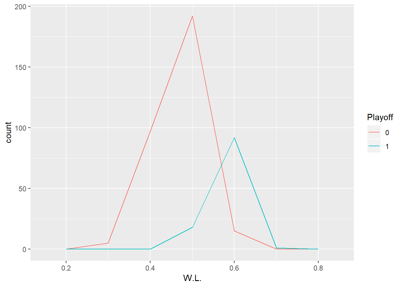

#correlation
data1 = as.data.frame(W.L.)
data1$Playoff <- as.numeric(data$Playoff)
data1$Champion <- data$Champion
data1$BA <- data$BA
data1$ERA <- data$ERA
data1$BatAge <- data$BatAge
data1$PAge <- data$PAge

corr <- round(cor(data1), 1)
ggcorrplot(corr, hc.order = TRUE, type = "lower", lab = TRUE)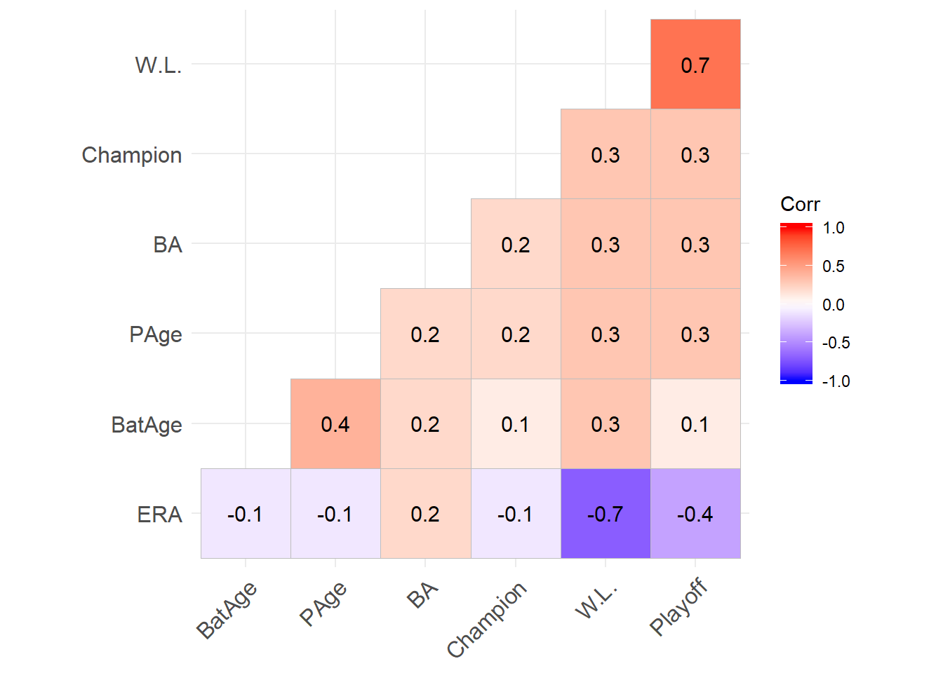

可以從第一個圖發現到進入季後賽之球隊例行賽普遍有較高的勝率，而第二張圖則呈現勝率與“是否進入季後賽”則有0.7的高相關性。

3.Linear Regression

在這個步驟，我會先建立一個全變數的模型，看一下是否有異狀，之後透過feature engineering，在考慮共線性的情況下，使用bestsubset的方法，建構最終模型，並進行殘差檢定。

3-1.fit full model

fit_lm <- lm(W.L.~.,data = data_lm)
summary(fit_lm)

## 
## Call:
## lm(formula = W.L. ~ ., data = data_lm)
## 
## Residuals:
##        Min         1Q     Median         3Q        Max 
## -0.0258200 -0.0071628  0.0008854  0.0059595  0.0303410 
## 
## Coefficients: (4 not defined because of singularities)
##               Estimate Std. Error t value Pr(>|t|)    
## (Intercept)  3.812e-01  1.673e+00   0.228 0.819938    
## X.Bat       -6.255e-06  2.294e-04  -0.027 0.978264    
## BatAge      -4.567e-04  5.923e-04  -0.771 0.441230    
## R.G         -1.907e-01  1.955e-01  -0.976 0.329918    
## G_x         -3.300e-03  7.360e-03  -0.448 0.654154    
## PA          -1.802e-03  3.955e-04  -4.557 7.11e-06 ***
## AB           1.258e-04  4.000e-04   0.315 0.753223    
## R_x          3.278e-03  1.221e-03   2.685 0.007579 ** 
## H_x         -2.891e-04  3.520e-04  -0.821 0.412055    
## X2B         -1.570e-04  2.354e-04  -0.667 0.505148    
## X3B         -2.821e-04  4.779e-04  -0.590 0.555325    
## HR_x        -3.317e-04  7.040e-04  -0.471 0.637789    
## RBI         -1.981e-04  9.497e-05  -2.086 0.037676 *  
## SB          -1.725e-05  2.545e-05  -0.678 0.498338    
## CS           9.449e-07  9.700e-05   0.010 0.992233    
## BB_x        -1.585e-04  4.263e-04  -0.372 0.710237    
## SO_x        -2.940e-06  7.363e-06  -0.399 0.689943    
## BA          -4.718e-01  1.725e+00  -0.274 0.784608    
## OBP         -1.477e+00  1.588e+00  -0.930 0.352903    
## SLG         -2.314e+00  1.566e+00  -1.478 0.140390    
## OPS          2.843e+00  1.241e+00   2.291 0.022509 *  
## OPS.         3.092e-04  2.989e-04   1.034 0.301625    
## TB                  NA         NA      NA       NA    
## GDP          8.377e-05  6.969e-05   1.202 0.230178    
## HBP_x       -1.229e-04  4.277e-04  -0.287 0.773959    
## SH           6.916e-06  3.989e-04   0.017 0.986176    
## SF           6.153e-05  4.213e-04   0.146 0.883985    
## IBB_x        1.451e-04  6.059e-05   2.394 0.017155 *  
## LOB_x        1.798e-03  8.676e-05  20.720  < 2e-16 ***
## X.P         -2.567e-04  2.852e-04  -0.900 0.368635    
## PAge         5.906e-05  5.546e-04   0.106 0.915249    
## RA.G         7.581e-02  1.827e-01   0.415 0.678476    
## ERA         -3.814e-02  1.555e-01  -0.245 0.806406    
## G_y                 NA         NA      NA       NA    
## GS                  NA         NA      NA       NA    
## GF           3.074e-04  3.379e-04   0.910 0.363505    
## CG                  NA         NA      NA       NA    
## tSho         6.715e-04  2.035e-04   3.300 0.001062 ** 
## cSho         1.653e-04  6.320e-04   0.262 0.793768    
## SV           4.945e-04  1.289e-04   3.837 0.000147 ***
## IP           1.956e-03  2.795e-03   0.700 0.484499    
## H_y         -1.268e-04  7.153e-04  -0.177 0.859398    
## R_y         -1.589e-03  1.508e-03  -1.054 0.292767    
## ER           2.284e-04  9.755e-04   0.234 0.815027    
## HR_y        -1.222e-04  1.584e-04  -0.772 0.440700    
## BB_y         2.533e-05  7.222e-04   0.035 0.972037    
## IBB_y       -2.517e-05  5.130e-05  -0.491 0.623996    
## SO_y        -7.279e-06  1.186e-04  -0.061 0.951073    
## HBP_y        2.325e-06  6.878e-05   0.034 0.973049    
## BK           4.189e-04  2.315e-04   1.809 0.071283 .  
## WP          -8.629e-05  4.892e-05  -1.764 0.078570 .  
## BF           1.126e-03  9.419e-04   1.195 0.232821    
## ERA.         7.599e-05  2.503e-04   0.304 0.761616    
## FIP         -9.007e-04  1.166e-02  -0.077 0.938449    
## WHIP         6.868e-02  1.018e+00   0.067 0.946240    
## H9           9.946e-03  1.998e-02   0.498 0.618957    
## HR9          1.773e-02  1.912e-02   0.927 0.354348    
## BB9         -1.960e-02  1.856e-02  -1.056 0.291687    
## SO9          4.051e-03  1.852e-02   0.219 0.827005    
## SO.W        -6.355e-03  9.076e-03  -0.700 0.484263    
## LOB_y       -1.119e-03  9.431e-04  -1.186 0.236286    
## ---
## Signif. codes:  0 '***' 0.001 '**' 0.01 '*' 0.05 '.' 0.1 ' ' 1
## 
## Residual standard error: 0.01065 on 363 degrees of freedom
## Multiple R-squared:  0.9789, Adjusted R-squared:  0.9756 
## F-statistic: 300.5 on 56 and 363 DF,  p-value: < 2.2e-16

Adjusted R-squared高達0.9756，但因解釋變數之間有高度相關性，因此模型還需要一些調整。

3-2.Vif func

透過fmsb套件，選取VIF < 10的變數出來。

vif_func<-function(in_frame,thresh=10,trace=T,...){

  library(fmsb)
  
  if(any(!'data.frame' %in% class(in_frame))) in_frame<-data.frame(in_frame)
  
  #get initial vif value for all comparisons of variables
  vif_init<-NULL
  var_names <- names(in_frame)
  for(val in var_names){
      regressors <- var_names[-which(var_names == val)]
      form <- paste(regressors, collapse = '+')
      form_in <- formula(paste(val, '~', form))
      vif_init<-rbind(vif_init, c(val, VIF(lm(form_in, data = in_frame, ...))))
      }
  vif_max<-max(as.numeric(vif_init[,2]), na.rm = TRUE)

  if(vif_max < thresh){
    if(trace==T){ #print output of each iteration
        prmatrix(vif_init,collab=c('var','vif'),rowlab=rep('',nrow(vif_init)),quote=F)
        cat('\n')
        cat(paste('All variables have VIF < ', thresh,', max VIF ',round(vif_max,2), sep=''),'\n\n')
        }
    return(var_names)
    }
  else{

    in_dat<-in_frame

    #backwards selection of explanatory variables, stops when all VIF values are below 'thresh'
    while(vif_max >= thresh){
      
      vif_vals<-NULL
      var_names <- names(in_dat)
        
      for(val in var_names){
        regressors <- var_names[-which(var_names == val)]
        form <- paste(regressors, collapse = '+')
        form_in <- formula(paste(val, '~', form))
        vif_add<-VIF(lm(form_in, data = in_dat, ...))
        vif_vals<-rbind(vif_vals,c(val,vif_add))
        }
      max_row<-which(vif_vals[,2] == max(as.numeric(vif_vals[,2]), na.rm = TRUE))[1]
      vif_max<-as.numeric(vif_vals[max_row,2])
      if(vif_max<thresh) break
      if(trace==T){ #print output of each iteration
        prmatrix(vif_vals,collab=c('var','vif'),rowlab=rep('',nrow(vif_vals)),quote=F)
        cat('\n')
        cat('removed: ',vif_vals[max_row,1],vif_max,'\n\n')
        flush.console()
        }
      in_dat<-in_dat[,!names(in_dat) %in% vif_vals[max_row,1]]
      }
    return(names(in_dat))
    }
  }
# my.stepwise
require(MASS)
require(clusterGeneration)
vif_func(in_frame=data_lm[,-32],thresh=5,trace=T)

ml1

3-3.Best subset

library(leaps)
regfit.best<-regsubsets(W.L.~X.Bat+BatAge+AB+X2B+X3B+HR_x+SB+CS+BB_x+SO_x+OPS.+GDP+HBP_x+SH+SF+IBB_x+X.P+PAge+CG+tSho+cSho+SV+IP+IBB_y+HBP_y+BK+WP+ERA.+HR9+BB9+SO9+LOB_y,data_lm,nvmax=15)
regsumm<-summary(regfit.best)

par(mfrow = c(2,2))
plot(regsumm$cp)
points(which.min(regsumm$cp), regsumm$cp[which.min(regsumm$cp)], col = "red", cex = 2, pch = 20)
plot(regsumm$rsq)
points(which.max(regsumm$rsq), regsumm$rsq[which.max(regsumm$rsq)], col = "red", cex = 2, pch = 20)
plot(regsumm$adjr2)
points(which.max(regsumm$adjr2), regsumm$adjr2[which.max(regsumm$adjr2)], col = "red", cex = 2, pch = 20)

fit_bestlm <- lm(W.L.~X.Bat + AB + HR_x + SO_x + OPS. + GDP + IBB_x + X.P + PAge +  tSho + SV+ IP+HBP_y+WP+ERA.,data_lm)
summary(fit_bestlm)

## 
## Call:
## lm(formula = W.L. ~ X.Bat + AB + HR_x + SO_x + OPS. + GDP + IBB_x + 
##     X.P + PAge + tSho + SV + IP + HBP_y + WP + ERA., data = data_lm)
## 
## Residuals:
##      Min       1Q   Median       3Q      Max 
## -0.06083 -0.01405  0.00036  0.01446  0.05646 
## 
## Coefficients:
##               Estimate Std. Error t value Pr(>|t|)    
## (Intercept) -5.342e-01  1.374e-01  -3.889 0.000118 ***
## X.Bat       -1.072e-03  4.183e-04  -2.562 0.010762 *  
## AB          -5.401e-05  2.076e-05  -2.602 0.009611 ** 
## HR_x         1.001e-04  4.438e-05   2.256 0.024592 *  
## SO_x        -3.741e-05  1.069e-05  -3.502 0.000514 ***
## OPS.         3.823e-03  2.013e-04  18.990  < 2e-16 ***
## GDP         -2.072e-04  7.728e-05  -2.681 0.007647 ** 
## IBB_x        3.558e-04  9.018e-05   3.946 9.38e-05 ***
## X.P          1.325e-03  5.240e-04   2.529 0.011819 *  
## PAge         2.978e-03  9.544e-04   3.120 0.001938 ** 
## tSho         1.489e-03  3.426e-04   4.346 1.75e-05 ***
## SV           2.321e-03  1.870e-04  12.414  < 2e-16 ***
## IP           3.510e-04  1.116e-04   3.145 0.001785 ** 
## HBP_y        1.921e-04  1.018e-04   1.888 0.059751 .  
## WP          -1.573e-04  8.545e-05  -1.841 0.066344 .  
## ERA.         3.110e-03  1.465e-04  21.225  < 2e-16 ***
## ---
## Signif. codes:  0 '***' 0.001 '**' 0.01 '*' 0.05 '.' 0.1 ' ' 1
## 
## Residual standard error: 0.02161 on 404 degrees of freedom
## Multiple R-squared:  0.9032, Adjusted R-squared:  0.8996 
## F-statistic: 251.3 on 15 and 404 DF,  p-value: < 2.2e-16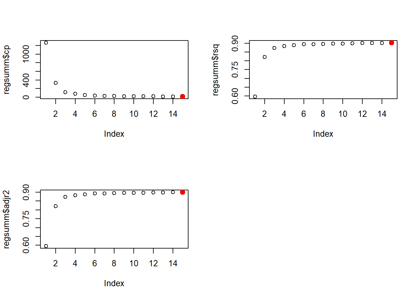

使用Best subset挑選上面通過VIF < 10的變數，並考慮各個選模準則後，以前15個變數建立最終模型。

3-4.Check vif

再次檢查模型共線性是否正常。

library(car)

## Loading required package: carData

## 
## Attaching package: 'car'

## The following object is masked from 'package:dplyr':
## 
##     recode

## The following object is masked from 'package:purrr':
## 
##     some

vif(fit_bestlm, digits = 3)

##    X.Bat       AB     HR_x     SO_x     OPS.      GDP    IBB_x      X.P 
## 3.716246 2.139950 2.130194 2.382842 2.054869 1.431635 1.271660 4.307475 
##     PAge     tSho       SV       IP    HBP_y       WP     ERA. 
## 1.297385 1.615041 1.538919 1.990054 1.203477 1.217617 2.181314

3-5.Residual

模型殘差檢定：

par(mfrow = c(2,2))
plot(fit_bestlm)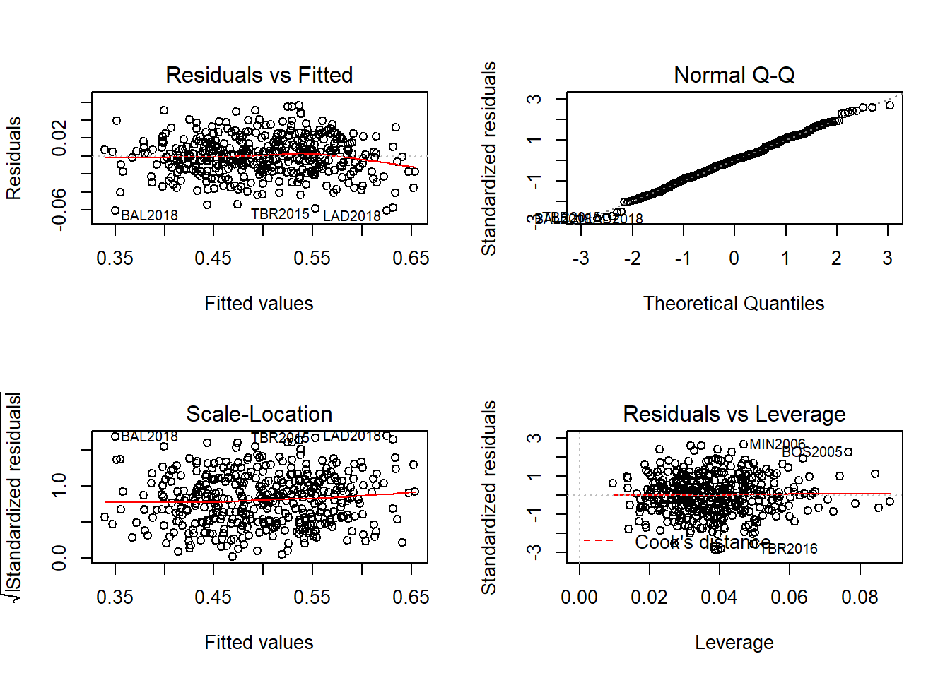

殘差分析結果：

正態性。當預測值固定時，因變量成正態分布，則殘差值也應該是一個均值為0的正態分布。正態QQ圖（Normal Q-Q，右上）是在正態分布對應的值下，標準化殘差的機率圖。若滿足正態假設，那麼圖上的點應該落在呈45度角的直線上；若不是如此，那麼久違反了正態性假設。
獨立性。因反應變數是各個年份的所有球隊勝率，因此多少有樣本間不獨立的問題，但因資料涵蓋多個年份，因此可減低同年互相影響的問題。
線性。若因變量與自變量線性相關，那麼殘差值與預測（擬合）值就沒有任何系統關聯。換句話說，除了白噪聲，模型應該包含數據中所有的系統方差，在「殘差圖與擬合圖」（Residual vs Fitted）中可以清楚的看到一個曲線關係，這暗示著你可能需要對回歸模型加上一個二次項。
同方差性。若滿足不變方差假設，那麼在位置尺度（Scale-Location Graph，左下）中，水平線周圍的點應該隨機分布。該圖似乎滿足此假設。

MLB win rate regression

Hermit