在這個資料中，我們有兩種細菌。前面的46個觀察值是CRE，後面的49個則不是。

我們希望將資料分類為是否為 CRE。Peak是蛋白質的名稱，而P_value是各蛋白質的重要程度，較低的p_value意味著對是否為CRE的影響更大。因此，我們將選取較低的p_value變數來構建分類器。

資料是水平資料。因此我們先將資料轉置成一個95個觀測值與1471個變數的格式，標記何者為CRE，然後使用機器學習方法對資料進行分類。最後，使用Leave-One-Out交叉驗證來比較各方法的測試精準度。

In this data, we have two types bacteria. The front 46 observers are CRE and back 49s are non-CRE.

We want to classificate the data to CRE or not. The p_value is the index of Peak(Protein types). Lower p_value means more influence for CREs. So we will pick lower p_value variables to build classificators.

The data is a horizontal data. So we will transpose the data become a size of 95 observations of 1471 variables at begining. Label the CREs ,then use machine learning methods to classificate data. Finally using the Leave-One-Out Cross Validation to compare methods’ test-accuracies.

Data processing

Read data

data_csv <- read.csv("C:\\Users\\User\\OneDrive - student.nsysu.edu.tw\\Educations\\NSYSU\\fu_chung\\bacterial\\20180111_CRE_46-non-CRE_49_Intensity.csv")

#preview the origin data
head(data_csv[,1:5],10)

##        Peak    p.value    q.value B1050328.154.CRE.KP B1050603.077.CRE.KP
## 1  1998.333 0.02145536 0.37130388                   0                0.00
## 2  2007.091 0.58751830 1.00000000                   0                0.00
## 3  2012.881 0.23143251 0.87068344                   0            11222.02
## 4  2030.663 0.60917531 1.00000000                   0                0.00
## 5  2036.960 1.00000000 1.00000000                   0                0.00
## 6  2059.762 1.00000000 1.00000000                   0                0.00
## 7  2090.549 0.67573691 1.00000000                   0           135239.75
## 8  2094.218 1.00000000 1.00000000                   0                0.00
## 9  2107.575 0.00045300 0.06658398                   0                0.00
## 10 2124.102 0.76943375 1.00000000                   0                0.00

可看出兩種類別的數量非常接近，CRE為46個，非CRE為49個。

arrange

將資料轉置成我們要的方向，因為原資料的peak有1471種，其重要性以p value的大小為分別，這裡我只取前50小(顯著)的種類，並且因為前面的46個觀察值是CRE，後面的49個則不是，因此在這裡幫前46比觀察值加入label，讓後續的分類可以更好進行。因此最終資料將呈現95比觀察值與51個變數(前50 peak 的解釋變數以及一個CRE類別反應變數)。

if (!require(tidyverse)) install.packages('tidyverse')

## Loading required package: tidyverse

## -- Attaching packages ----------------------------------------------------------------------------------------------- tidyverse 1.2.1 --

## √ ggplot2 3.1.1       √ purrr   0.3.2  
## √ tibble  2.1.1       √ dplyr   0.8.0.1
## √ tidyr   0.8.3       √ stringr 1.4.0  
## √ readr   1.3.1       √ forcats 0.4.0

## -- Conflicts -------------------------------------------------------------------------------------------------- tidyverse_conflicts() --
## x dplyr::filter() masks stats::filter()
## x dplyr::lag()    masks stats::lag()

library(tidyverse)

#sort data by p.value
data_csv <- arrange(data_csv,p.value)

#transpose data
name_protein <- data_csv[,1]
data <- as.data.frame(t(data_csv))
data <- data[-c(1:3),]

#remain 50 variables who have the lower p.value
name_variable <- names(data)
data <- data[,c(1:50)]

#data name
data_name <- data.frame(name_variable,name_protein)
data_name <- as.data.frame(t(data_name))
head(data_name[1:5])

##                      V1        V2        V3        V4        V5
## name_variable        V1        V2        V3        V4        V5
## name_protein   2636.880  3830.576  4447.421  3317.308  7401.614

#label CRE as factor
data$CRE <- as.factor(c(rep(1,46),rep(0,49)))

#preview front of 5 variables and CRE.
head(data[,c(1:5,51)],10)

##                           V1        V2        V3       V4       V5 CRE
## B1050328.154.CRE.KP 251357.7      0.00  494285.5 114879.4 31439.26   1
## B1050603.077.CRE.KP 394550.2  65408.65 2186094.8 137296.9     0.00   1
## B1050723.021.CRE.KP      0.0 129236.21  675608.8 182865.2 16074.49   1
## B1050902.121.CRE.KP 137403.3      0.00  818021.2      0.0     0.00   1
## B1060202.094.CRE.KP 377358.8 327564.66  532502.6      0.0     0.00   1
## B1060217.087.CRE.KP 321700.3 300239.31  220649.5 289622.5 42589.68   1
## B1060311.004.CRE.KP 122302.3 163517.28  143966.8 197686.0 44586.54   1
## B1060429.067.CRE.KP 458382.1 136389.20  412460.2 294669.0 46850.84   1
## B1060522.013.CRE.KP 404748.2  97165.77  800137.4 134355.1     0.00   1
## B1060606.077.CRE.KP      0.0 237456.30  489450.3 317787.7     0.00   1

#Plot the CRE type
plot(data$CRE)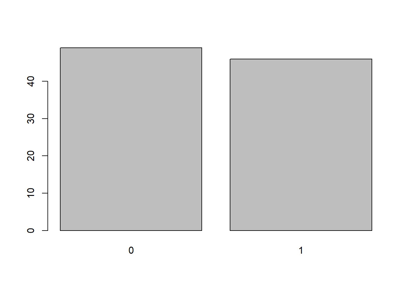

Bulid the Classificators

Support vector machine

if (!require(e1071)) install.packages('e1071')

## Loading required package: e1071

library(e1071)

svm_loocv_accuracy <- vector()

for(i in c(1:95)){
  train = data[-i, ]
  test  = data[i, ] 

  svm_model = svm(formula = CRE ~ ., 
            data = train)
  
  test.pred = predict(svm_model, test)

  #Accuracy
  confus.matrix = table(real=test$CRE, predict=test.pred)
  svm_loocv_accuracy[i]=sum(diag(confus.matrix))/sum(confus.matrix)
}

#LOOCV test accuracy
mean(svm_loocv_accuracy) # Accurary with LOOCV = 0.8526316

## [1] 0.8526316

Random Forest

if (!require(randomForest)) install.packages('randomForest')

## Loading required package: randomForest

## randomForest 4.6-14

## Type rfNews() to see new features/changes/bug fixes.

## 
## Attaching package: 'randomForest'

## The following object is masked from 'package:dplyr':
## 
##     combine

## The following object is masked from 'package:ggplot2':
## 
##     margin

library(randomForest)

rf_loocv_accuracy <- vector()

for(i in c(1:95)){
  train = data[-i, ]
  test  = data[i, ]

  rf_model = randomForest(CRE~.,
                        data=train,
                        ntree=150        # num of decision Tree
                        )
  
  test.pred = predict(rf_model, test)

  #Accuracy
  confus.matrix = table(real=test$CRE, predict=test.pred)
  rf_loocv_accuracy[i]=sum(diag(confus.matrix))/sum(confus.matrix)
}

#LOOCV test accuracy
mean(rf_loocv_accuracy) # Accurary with LOOCV = 0.9157895

## [1] 0.8947368

KNN with distance = 10

if (!require(kknn))install.packages("kknn")

## Loading required package: kknn

library(kknn)

knn_loocv_accuracy <- vector()
for(i in c(1:95)){
  train = data[-i, ]
  test  = data[i, ]

  knn_model <- kknn(CRE~., train, test, distance = 10)   # knn distance = 10
  
  fit <- fitted(knn_model)

  #Accuracy
  confus.matrix = table(real=test$CRE, predict=test.pred)
  knn_loocv_accuracy[i]=sum(diag(confus.matrix))/sum(confus.matrix)
  
}

#LOOCV test accuracy
mean(knn_loocv_accuracy) # Accurary with LOOCV = 0.5157895

## [1] 0.5157895

Naïve Bayes

if (!require(e1071))install.packages("e1071")
library(e1071)

nb_loocv_accuracy <- vector()
nb_loocv_mse <- vector()

for(i in c(1:95)){
  train = data[-i, ]
  test  = data[i, ]

  nb_model=naiveBayes(CRE~., data=train)
  
  test.pred = predict(nb_model, test)
  
  #Accuracy
  confus.matrix = table(test$CRE, test.pred)
  nb_loocv_accuracy[i] <- sum(diag(confus.matrix))/sum(confus.matrix)
}

#LOOCV test accuracy
mean(nb_loocv_accuracy) # Accurary with LOOCV = 0.6947368

## [1] 0.6947368

Logistic Regression

lr_loocv_accuracy <- vector()
for(i in c(1:95)){
  train = data[-i, ]
  test  = data[i, ]

  lr_model<-glm(formula=CRE~.,data=train, family=binomial(link="logit"),na.action=na.exclude)
  
  test.pred = predict(lr_model, test)

  #Accuracy
  confus.matrix = table(test$CRE, test.pred)
  lr_loocv_accuracy[i] <- sum(diag(confus.matrix))/sum(confus.matrix)
}

#LOOCV test accuracy
mean(lr_loocv_accuracy) # Accurary with LOOCV = 0.5157895

## [1] 0.5157895

The LOOCV Accuracy rank for this data is :
1. “Random Forest(0.9157895)”
2. “Support vector machine(0.8526316)”
3. “Naïve Bayes(0.6947368)”
4. “Logistic Regression(0.5157895)”
4. “KNN = 10 (0.5157895)”

CRE Bacteria Data Analysis

Hermit