這次我使用sklearn內建的資料集breast-cancer(原始資料來源：https://archive.ics.uci.edu/ml/datasets/Breast+Cancer+Wisconsin+(Diagnostic)) ，先將原資料以7:3比例建立一個的資料分類器出來，之後把其中一個類別挑出，並使用各種oversampling的方法來模擬樣本，並最終將模擬後的資料套回最初的模型當中，比較各方法產生的樣本能否在分類器當中回到原本的類別當中。

1. 讀入資料

讀取sklearn的資料並轉為dataframe：

import pandas as pd
import numpy as np
from sklearn import datasets

# import some data to play with
df = datasets.load_breast_cancer()
x = pd.DataFrame(df['data'],columns = df['feature_names'])
y = pd.DataFrame(df['target'],columns = ['targets_names'])

稍微檢查一下資料的型態與內容：

print(x.shape)
x.head()

(569, 30)

	mean radius	mean texture	mean perimeter	mean area	mean smoothness	mean compactness	mean concavity	mean concave points	mean symmetry	mean fractal dimension	…	worst radius	worst texture	worst perimeter	worst area	worst smoothness	worst compactness	worst concavity	worst concave points	worst symmetry	worst fractal dimension
0	17.99	10.38	122.80	1001.0	0.11840	0.27760	0.3001	0.14710	0.2419	0.07871	…	25.38	17.33	184.60	2019.0	0.1622	0.6656	0.7119	0.2654	0.4601	0.11890
1	20.57	17.77	132.90	1326.0	0.08474	0.07864	0.0869	0.07017	0.1812	0.05667	…	24.99	23.41	158.80	1956.0	0.1238	0.1866	0.2416	0.1860	0.2750	0.08902
2	19.69	21.25	130.00	1203.0	0.10960	0.15990	0.1974	0.12790	0.2069	0.05999	…	23.57	25.53	152.50	1709.0	0.1444	0.4245	0.4504	0.2430	0.3613	0.08758
3	11.42	20.38	77.58	386.1	0.14250	0.28390	0.2414	0.10520	0.2597	0.09744	…	14.91	26.50	98.87	567.7	0.2098	0.8663	0.6869	0.2575	0.6638	0.17300
4	20.29	14.34	135.10	1297.0	0.10030	0.13280	0.1980	0.10430	0.1809	0.05883	…	22.54	16.67	152.20	1575.0	0.1374	0.2050	0.4000	0.1625	0.2364	0.07678

5 rows × 30 columns

y.head()

	targets_names
0	0
1	0
2	0
3	0
4	0

%matplotlib inline
by_fraud = y.groupby('targets_names')
by_fraud.size().plot(kind = 'bar')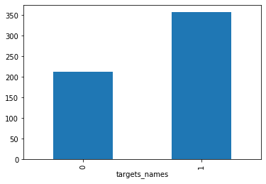

2. 建構分類器

這次使用adaboost來建立分類器，其準確率大約為0.99-0.95之間。

from sklearn.model_selection import train_test_split
from sklearn.ensemble import AdaBoostClassifier
from sklearn import ensemble
from sklearn import metrics
import random

random.seed(1)
arr = np.arange(569)
np.random.shuffle(arr)


train_X = x.iloc[arr[0:398],:]
test_X = x.iloc[arr[398:569],:]
train_y = y.iloc[arr[0:398],:]
test_y = y.iloc[arr[398:569],:]

clf = AdaBoostClassifier(n_estimators=100)
#forest = ensemble.RandomForestClassifier(n_estimators = 100)
fit = clf.fit(train_X, train_y)

test_y_predicted = clf.predict(test_X)
accuracy_rf = metrics.accuracy_score(test_y, test_y_predicted)
print(accuracy_rf)

C:3-gpu-packages.py:724: DataConversionWarning: A column-vector y was passed when a 1d array was expected. Please change the shape of y to (n_samples, ), for example using ravel(). y = column_or_1d(y, warn=True)

0.9941520467836257

3. 生成資料

將0類(較少類)資料切出，並使用ocwgan,ocgan,smote與adasyn等方法，在此先設定這些方法：

f_x = x[y['targets_names'].isin([0])]
f_y = y[y['targets_names'].isin([0])]
print(f_x.shape)
print(f_y.shape)

(212, 30) (212, 1)

f_x.head()

	mean radius	mean texture	mean perimeter	mean area	mean smoothness	mean compactness	mean concavity	mean concave points	mean symmetry	mean fractal dimension	…	worst radius	worst texture	worst perimeter	worst area	worst smoothness	worst compactness	worst concavity	worst concave points	worst symmetry	worst fractal dimension
0	17.99	10.38	122.80	1001.0	0.11840	0.27760	0.3001	0.14710	0.2419	0.07871	…	25.38	17.33	184.60	2019.0	0.1622	0.6656	0.7119	0.2654	0.4601	0.11890
1	20.57	17.77	132.90	1326.0	0.08474	0.07864	0.0869	0.07017	0.1812	0.05667	…	24.99	23.41	158.80	1956.0	0.1238	0.1866	0.2416	0.1860	0.2750	0.08902
2	19.69	21.25	130.00	1203.0	0.10960	0.15990	0.1974	0.12790	0.2069	0.05999	…	23.57	25.53	152.50	1709.0	0.1444	0.4245	0.4504	0.2430	0.3613	0.08758
3	11.42	20.38	77.58	386.1	0.14250	0.28390	0.2414	0.10520	0.2597	0.09744	…	14.91	26.50	98.87	567.7	0.2098	0.8663	0.6869	0.2575	0.6638	0.17300
4	20.29	14.34	135.10	1297.0	0.10030	0.13280	0.1980	0.10430	0.1809	0.05883	…	22.54	16.67	152.20	1575.0	0.1374	0.2050	0.4000	0.1625	0.2364	0.07678

5 rows × 30 columns

3.1 OCWGAN setting

# import modules
%matplotlib inline
import os
import random
import keras
import numpy as np
import pandas as pd
import matplotlib.pyplot as plt
import seaborn as sns
from tqdm import tqdm_notebook as tqdm
from keras.models import Model
from keras.layers import Input, Reshape
from keras.layers.core import Dense, Activation, Dropout, Flatten
from keras.layers.normalization import BatchNormalization
from keras.layers.convolutional import UpSampling1D, Conv1D
from keras.layers.advanced_activations import LeakyReLU
from keras.optimizers import Adam, SGD,RMSprop
from keras.callbacks import TensorBoard
from sklearn.preprocessing import StandardScaler

# set parameters
dim = f_x.shape[1]
num = f_x.shape[0]
g_data = f_x

# Standard Scaler
ss = StandardScaler()
g_data = pd.DataFrame(ss.fit_transform(g_data))

# wasserstein_loss
from keras import backend 
# implementation of wasserstein loss
def wasserstein_loss(y_true, y_pred):
    return backend.mean(y_true * y_pred)

# generator
def get_generative(G_in, dense_dim=200, out_dim= dim, lr=1e-3):
    x = Dense(dense_dim)(G_in)
    x = Activation('tanh')(x)
    G_out = Dense(out_dim, activation='tanh')(x)
    G = Model(G_in, G_out)
    opt = keras.optimizers.RMSprop(lr=lr)#原先為SGD
    G.compile(loss=wasserstein_loss, optimizer=opt)#原loss為binary_crossentropy
    return G, G_out

G_in = Input(shape=[10])
G, G_out = get_generative(G_in)
G.summary()

# discriminator
def get_discriminative(D_in, lr=1e-3, drate=.25, n_channels= dim, conv_sz=5, leak=.2):#lr=1e-3, drate=.25, n_channels= dim, conv_sz=5, leak=.2
    x = Reshape((-1, 1))(D_in)
    x = Conv1D(n_channels, conv_sz, activation='relu')(x)
    x = Dropout(drate)(x)
    x = Flatten()(x)
    x = Dense(n_channels)(x)
    D_out = Dense(2, activation='linear')(x)#sigmoid
    D = Model(D_in, D_out)
    dopt = keras.optimizers.RMSprop(lr=lr)#原先為Adam
    D.compile(loss=wasserstein_loss, optimizer=dopt)
    return D, D_out

D_in = Input(shape=[dim])
D, D_out = get_discriminative(D_in)
D.summary()

# set up gan
def set_trainability(model, trainable=False):
    model.trainable = trainable
    for layer in model.layers:
        layer.trainable = trainable
        
def make_gan(GAN_in, G, D):
    set_trainability(D, False)
    x = G(GAN_in)
    GAN_out = D(x)
    GAN = Model(GAN_in, GAN_out)
    GAN.compile(loss=wasserstein_loss, optimizer=G.optimizer)#元loss為binary_crossentropy
    return GAN, GAN_out

GAN_in = Input([10])
GAN, GAN_out = make_gan(GAN_in, G, D)
GAN.summary()

# pre train
def sample_data_and_gen(G, noise_dim=10, n_samples= num):
    XT = np.array(g_data)
    XN_noise = np.random.uniform(0, 1, size=[n_samples, noise_dim])
    XN = G.predict(XN_noise)
    X = np.concatenate((XT, XN))
    y = np.zeros((2*n_samples, 2))
    y[:n_samples, 1] = 1
    y[n_samples:, 0] = 1
    return X, y

def pretrain(G, D, noise_dim=10, n_samples = num, batch_size=32):
    X, y = sample_data_and_gen(G, n_samples=n_samples, noise_dim=noise_dim)
    set_trainability(D, True)
    D.fit(X, y, epochs=1, batch_size=batch_size)
    
pretrain(G, D)

def sample_noise(G, noise_dim=10, n_samples=num):
    X = np.random.uniform(0, 1, size=[n_samples, noise_dim])
    y = np.zeros((n_samples, 2))
    y[:, 1] = 1
    return X, y

# one class detector
def oneclass(data,kernel = 'rbf',gamma = 'auto'):
    num1 = int(len(data)/2)
    num2 = int(len(data)+1)
    from sklearn import svm
    clf = svm.OneClassSVM(kernel=kernel, gamma=gamma).fit(data[0:num1])
    origin = pd.DataFrame(clf.score_samples(data[0:num1]))
    new = pd.DataFrame(clf.score_samples(data[num1:num2]))

    occ = pd.concat([pd.DataFrame(new[0] < origin[0].min()),pd.DataFrame(new[0] > origin[0].max())], axis=1)
    occ['ava'] = pd.DataFrame(occ.iloc[:,1:2] == occ.iloc[:,0:1])
    err = sum(occ['ava'] == False)/len(occ['ava'])
    return err

# productor
def gen(GAN, G, D, times=50, n_samples= num, noise_dim=10, batch_size=32, verbose=False, v_freq=dim,):
    data = pd.DataFrame()
    for epoch in range(times):
        X, y = sample_data_and_gen(G, n_samples=n_samples, noise_dim=noise_dim)
        set_trainability(D, True)   
        xx,yy = X,y
        err = oneclass(xx)        
        num1 = int(len(xx)/2)
        num2 = int(len(xx)+1)
        xx = ss.inverse_transform(xx)
        data = pd.concat([data,pd.DataFrame(xx[num1:num2])],axis = 0)              
        print("The %d times generator one class svm Error Rate=%f" %(epoch, err))           
            
    return data

# training
def train(GAN, G, D, epochs=1, n_samples= num, noise_dim=10, batch_size=32, verbose=False, v_freq=dim,):
    d_loss = []
    g_loss = []
    e_range = range(epochs)
    if verbose:
        e_range = tqdm(e_range)
    for epoch in e_range:
        X, y = sample_data_and_gen(G, n_samples=n_samples, noise_dim=noise_dim)
        set_trainability(D, True)
        d_loss.append(D.train_on_batch(X, y))
        xx,yy = X,y
        err = oneclass(xx) 
        print("The %d times epoch one class svm Error Rate=%f" %(epoch, err))
        
        X, y = sample_noise(G, n_samples=n_samples, noise_dim=noise_dim)
        set_trainability(D, False)
        g_loss.append(GAN.train_on_batch(X, y))
        if verbose and (epoch + 1) % v_freq == 0:
            print("Epoch #{}: Generative Loss: {}, Discriminative Loss: {}".format(epoch + 1, g_loss[-1], d_loss[-1]))       
            
    return d_loss, g_loss, xx, yy

Layer (type) Output Shape Param #
================================================================= input_25 (InputLayer) (None, 10) 0
_________________________________________________________________ dense_27 (Dense) (None, 200) 2200
_________________________________________________________________ activation_12 (Activation) (None, 200) 0
_________________________________________________________________ dense_28 (Dense) (None, 30) 6030
================================================================= Total params: 8,230 Trainable params: 8,230 Non-trainable params: 0 _________________________________________________________________ _________________________________________________________________ Layer (type) Output Shape Param #
================================================================= input_26 (InputLayer) (None, 30) 0
_________________________________________________________________ reshape_12 (Reshape) (None, 30, 1) 0
_________________________________________________________________ conv1d_12 (Conv1D) (None, 26, 30) 180
_________________________________________________________________ dropout_12 (Dropout) (None, 26, 30) 0
_________________________________________________________________ flatten_12 (Flatten) (None, 780) 0
_________________________________________________________________ dense_29 (Dense) (None, 30) 23430
_________________________________________________________________ dense_30 (Dense) (None, 2) 62
================================================================= Total params: 23,672 Trainable params: 23,672 Non-trainable params: 0 _________________________________________________________________ _________________________________________________________________ Layer (type) Output Shape Param #
================================================================= input_27 (InputLayer) (None, 10) 0
_________________________________________________________________ model_16 (Model) (None, 30) 8230
_________________________________________________________________ model_17 (Model) (None, 2) 23672
================================================================= Total params: 31,902 Trainable params: 8,230 Non-trainable params: 23,672 _________________________________________________________________ Epoch 1/1 424/424 [==============================] - ETA: 5s - loss: 0.005 - 1s 1ms/step - loss: -1.6706

3.2 OCGAN setting

# import modules
%matplotlib inline
import os
import random
import numpy as np
import pandas as pd
import matplotlib.pyplot as plt
import seaborn as sns
from tqdm import tqdm_notebook as tqdm
from keras.models import Model
from keras.layers import Input, Reshape
from keras.layers.core import Dense, Activation, Dropout, Flatten
from keras.layers.normalization import BatchNormalization
from keras.layers.convolutional import UpSampling1D, Conv1D
from keras.layers.advanced_activations import LeakyReLU
from keras.optimizers import Adam, SGD
from keras.callbacks import TensorBoard
from sklearn.preprocessing import StandardScaler

# set parameters
dim = f_x.shape[1]
num = f_x.shape[0]
g_data = f_x

# Standard Scaler
ss = StandardScaler()
g_data = pd.DataFrame(ss.fit_transform(g_data))

# generator
def get_generative(G_in, dense_dim=200, out_dim= dim, lr=1e-3):
    x = Dense(dense_dim)(G_in)
    x = Activation('tanh')(x)
    G_out = Dense(out_dim, activation='tanh')(x)
    G = Model(G_in, G_out)
    opt = SGD(lr=lr)
    G.compile(loss='binary_crossentropy', optimizer=opt)
    return G, G_out

G_in = Input(shape=[10])
G, G_out = get_generative(G_in)
G.summary()

# discriminator
def get_discriminative(D_in, lr=1e-3, drate=.25, n_channels= dim, conv_sz=5, leak=.2):
    x = Reshape((-1, 1))(D_in)
    x = Conv1D(n_channels, conv_sz, activation='relu')(x)
    x = Dropout(drate)(x)
    x = Flatten()(x)
    x = Dense(n_channels)(x)
    D_out = Dense(2, activation='sigmoid')(x)
    D = Model(D_in, D_out)
    dopt = Adam(lr=lr)
    D.compile(loss='binary_crossentropy', optimizer=dopt)
    return D, D_out

D_in = Input(shape=[dim])
D, D_out = get_discriminative(D_in)
D.summary()

# set up gan
def set_trainability(model, trainable=False):
    model.trainable = trainable
    for layer in model.layers:
        layer.trainable = trainable
        
def make_gan(GAN_in, G, D):
    set_trainability(D, False)
    x = G(GAN_in)
    GAN_out = D(x)
    GAN = Model(GAN_in, GAN_out)
    GAN.compile(loss='binary_crossentropy', optimizer=G.optimizer)
    return GAN, GAN_out

GAN_in = Input([10])
GAN, GAN_out = make_gan(GAN_in, G, D)
GAN.summary()

# pre train
def sample_data_and_gen(G, noise_dim=10, n_samples= num):
    XT = np.array(g_data)
    XN_noise = np.random.uniform(0, 1, size=[n_samples, noise_dim])
    XN = G.predict(XN_noise)
    X = np.concatenate((XT, XN))
    y = np.zeros((2*n_samples, 2))
    y[:n_samples, 1] = 1
    y[n_samples:, 0] = 1
    return X, y

def pretrain(G, D, noise_dim=10, n_samples = num, batch_size=32):
    X, y = sample_data_and_gen(G, n_samples=n_samples, noise_dim=noise_dim)
    set_trainability(D, True)
    D.fit(X, y, epochs=1, batch_size=batch_size)
    
pretrain(G, D)

def sample_noise(G, noise_dim=10, n_samples=num):
    X = np.random.uniform(0, 1, size=[n_samples, noise_dim])
    y = np.zeros((n_samples, 2))
    y[:, 1] = 1
    return X, y

# one class detector
def oneclass(data,kernel = 'rbf',gamma = 'auto'):
    num1 = int(len(data)/2)
    num2 = int(len(data)+1)
    from sklearn import svm
    clf = svm.OneClassSVM(kernel=kernel, gamma=gamma).fit(data[0:num1])
    origin = pd.DataFrame(clf.score_samples(data[0:num1]))
    new = pd.DataFrame(clf.score_samples(data[num1:num2]))

    occ = pd.concat([pd.DataFrame(new[0] < origin[0].min()),pd.DataFrame(new[0] > origin[0].max())], axis=1)
    occ['ava'] = pd.DataFrame(occ.iloc[:,1:2] == occ.iloc[:,0:1])
    err = sum(occ['ava'] == False)/len(occ['ava'])
    return err

# training
def train1(GAN, G, D, epochs=1, n_samples= num, noise_dim=10, batch_size=32, verbose=False, v_freq=dim,):
    d_loss = []
    g_loss = []
    e_range = range(epochs)
    if verbose:
        e_range = tqdm(e_range)
    for epoch in e_range:
        X, y = sample_data_and_gen(G, n_samples=n_samples, noise_dim=noise_dim)
        set_trainability(D, True)
        d_loss.append(D.train_on_batch(X, y))
        xx,yy = X,y
        err = oneclass(xx) 
        print("The %d times epoch one class svm Error Rate=%f" %(epoch, err))
        
        X, y = sample_noise(G, n_samples=n_samples, noise_dim=noise_dim)
        set_trainability(D, False)
        g_loss.append(GAN.train_on_batch(X, y))
        if verbose and (epoch + 1) % v_freq == 0:
            print("Epoch #{}: Generative Loss: {}, Discriminative Loss: {}".format(epoch + 1, g_loss[-1], d_loss[-1]))
    return d_loss, g_loss, xx, yy

Layer (type) Output Shape Param #
================================================================= input_28 (InputLayer) (None, 10) 0
_________________________________________________________________ dense_31 (Dense) (None, 200) 2200
_________________________________________________________________ activation_13 (Activation) (None, 200) 0
_________________________________________________________________ dense_32 (Dense) (None, 30) 6030
================================================================= Total params: 8,230 Trainable params: 8,230 Non-trainable params: 0 _________________________________________________________________ _________________________________________________________________ Layer (type) Output Shape Param #
================================================================= input_29 (InputLayer) (None, 30) 0
_________________________________________________________________ reshape_13 (Reshape) (None, 30, 1) 0
_________________________________________________________________ conv1d_13 (Conv1D) (None, 26, 30) 180
_________________________________________________________________ dropout_13 (Dropout) (None, 26, 30) 0
_________________________________________________________________ flatten_13 (Flatten) (None, 780) 0
_________________________________________________________________ dense_33 (Dense) (None, 30) 23430
_________________________________________________________________ dense_34 (Dense) (None, 2) 62
================================================================= Total params: 23,672 Trainable params: 23,672 Non-trainable params: 0 _________________________________________________________________ _________________________________________________________________ Layer (type) Output Shape Param #
================================================================= input_30 (InputLayer) (None, 10) 0
_________________________________________________________________ model_19 (Model) (None, 30) 8230
_________________________________________________________________ model_20 (Model) (None, 2) 23672
================================================================= Total params: 31,902 Trainable params: 8,230 Non-trainable params: 23,672 _________________________________________________________________ Epoch 1/1 424/424 [==============================] - ETA: 9s - loss: 0.726 - 1s 2ms/step - loss: 0.5255

3.3 SMOTE setting

from imblearn.over_sampling import SMOTE
smo = SMOTE()
X_smo, y_smo = smo.fit_sample(x, y)
X_smo = pd.DataFrame(X_smo)
y_smo = pd.DataFrame(y_smo)

%matplotlib inline
by_fraud = y_smo.groupby(0)
by_fraud.size().plot(kind = 'bar')

<matplotlib.axes._subplots.AxesSubplot at 0x27f27709dd8>

3. 4 ADASYN setting

from imblearn.over_sampling import ADASYN
ada = ADASYN()
X_ada, y_ada = ada.fit_sample(x, y)
X_ada = pd.DataFrame(X_ada)
y_ada = pd.DataFrame(y_ada)

4. 比較效果

我們將生成後的資料丟入之前建立的分類器當中，並希望其落於’0’類別，我會計算出現1的比例，比例越低代表越好，以下是個方法結果：

4.1 OCWGAN

我將不同的one class svm Error Rate做分類，欲比較其差異的效果。 ### ocwgan epoch 1

d_loss, g_loss ,xx,yy= train(GAN, G, D, epochs=1, verbose=True)
new_data = gen(GAN, G, D, times = 1,verbose=True)
test_y_predicted = clf.predict(new_data)
print(test_y_predicted,'error = ',np.mean(test_y_predicted))

The 0 times epoch one class svm Error Rate=1.000000

The 0 times generator one class svm Error Rate=0.896226 [0 0 0 0 0 0 0 0 0 0 0 0 0 0 0 0 0 0 0 0 0 0 0 0 0 0 0 0 0 0 0 0 0 0 0 0 0 0 0 0 0 0 0 0 0 0 0 0 0 0 0 0 0 0 0 0 0 0 0 0 0 0 0 0 0 0 0 0 0 0 0 0 0 0 0 0 0 0 0 0 0 0 0 0 0 0 0 0 0 0 0 0 0 0 0 0 0 0 0 0 0 0 0 0 0 0 0 0 0 0 0 0 0 0 0 0 0 0 0 0 0 0 0 0 0 0 0 0 0 0 0 0 0 0 0 0 0 0 0 0 0 0 0 0 0 0 0 0 0 0 0 0 0 0 0 0 0 0 0 0 0 0 0 0 0 0 0 0 0 0 0 0 0 0 0 0 0 0 0 0 0 0 0 0 0 0 0 0 0 0 0 0 0 0 0 0 0 0 0 0 0 0 0 0 0 0 0 0 0 0 0 0]
error = 0.0

ocwgan epoch 2

d_loss, g_loss ,xx,yy= train(GAN, G, D, epochs=1, verbose=True)
new_data = gen(GAN, G, D, times = 1,verbose=True)
test_y_predicted = clf.predict(new_data)
test_y_predicted
print(test_y_predicted,'error = ',np.mean(test_y_predicted))

The 0 times epoch one class svm Error Rate=0.853774

The 0 times generator one class svm Error Rate=0.240566 [0 0 0 0 0 0 0 0 0 0 0 0 0 0 0 0 0 0 0 0 0 0 0 0 0 0 0 0 0 0 0 0 0 0 0 0 0 0 0 0 0 0 0 0 0 0 0 0 0 0 0 0 0 0 0 0 0 0 0 0 0 0 0 0 0 0 0 0 0 0 0 0 0 0 0 0 0 0 0 0 0 0 0 0 0 0 0 0 0 0 0 0 0 0 0 0 0 0 0 0 0 0 0 0 0 0 0 0 0 0 0 0 0 0 0 0 0 0 0 0 0 0 0 0 0 0 0 0 0 0 0 0 0 0 0 0 0 0 0 0 0 0 0 0 0 0 0 0 0 0 0 0 0 0 0 0 0 0 0 0 0 0 0 0 0 0 0 0 0 0 0 0 0 0 0 0 0 0 0 0 0 0 0 0 0 0 0 0 0 0 0 0 0 0 0 0 0 0 0 0 0 0 0 0 0 0 0 0 0 0 0 0]
error = 0.0