這次,我將使用一個來自kaggle的不平衡數據資料(link:https://www.kaggle.com/mlg-ulb/creditcardfraud/version/1).

該數據集包含了歐洲持卡人2013年9月通過信用卡進行的交易。這些交易發生在兩天之內,在這裡我們有492筆詐騙資料以及284807正常交易資料。該數據集是非常不平衡的,其中陰性樣本(詐欺)佔所有交易的0.172%。它的變量包含數值輸入變量後PCA變換的結果。不幸的是,由於保密問題我們不能得到原始數據的更多背景信息。特徵V1,V2,…… V28與PCA獲得的主成分,還沒有被轉化與PCA的變量是“交易時間”和“交易金額”。特徵“時間”為與第一筆交易所間隔的時間(秒)。特徵“金額”是交易金額,該功能可以被用於例如依賴性成本靈敏學習。特徵“class”是反應變量,並將其在欺詐的情況下取值為1。
而這次我的主要目的是,用數種常見的採樣方法與gan的過採樣方法進行簡單的比較,以平衡後的數據對其做相同的分類機器學習,這裡一慮採用random forest(n = 100)來建立分類器,屆時比較各採樣方法的accuracy與auc。
Data Visualization
在這裡我會做一些資料的切割以及簡單的視覺化,提供一些資料的簡單資訊。
import pandas as pd
import numpy as np

df = pd.read_csv('C:/Users/User/OneDrive - student.nsysu.edu.tw/Documents/dataset/creditcard.csv')
fraud = df[df['Class'].isin([1])]
normal = df[df['Class'].isin([0])]
df.head()| Time | V1 | V2 | V3 | V4 | V5 | V6 | V7 | V8 | V9 | … | V21 | V22 | V23 | V24 | V25 | V26 | V27 | V28 | Amount | Class | |
|---|---|---|---|---|---|---|---|---|---|---|---|---|---|---|---|---|---|---|---|---|---|
| 0 | 0.0 | -1.359807 | -0.072781 | 2.536347 | 1.378155 | -0.338321 | 0.462388 | 0.239599 | 0.098698 | 0.363787 | … | -0.018307 | 0.277838 | -0.110474 | 0.066928 | 0.128539 | -0.189115 | 0.133558 | -0.021053 | 149.62 | 0 |
| 1 | 0.0 | 1.191857 | 0.266151 | 0.166480 | 0.448154 | 0.060018 | -0.082361 | -0.078803 | 0.085102 | -0.255425 | … | -0.225775 | -0.638672 | 0.101288 | -0.339846 | 0.167170 | 0.125895 | -0.008983 | 0.014724 | 2.69 | 0 |
| 2 | 1.0 | -1.358354 | -1.340163 | 1.773209 | 0.379780 | -0.503198 | 1.800499 | 0.791461 | 0.247676 | -1.514654 | … | 0.247998 | 0.771679 | 0.909412 | -0.689281 | -0.327642 | -0.139097 | -0.055353 | -0.059752 | 378.66 | 0 |
| 3 | 1.0 | -0.966272 | -0.185226 | 1.792993 | -0.863291 | -0.010309 | 1.247203 | 0.237609 | 0.377436 | -1.387024 | … | -0.108300 | 0.005274 | -0.190321 | -1.175575 | 0.647376 | -0.221929 | 0.062723 | 0.061458 | 123.50 | 0 |
| 4 | 2.0 | -1.158233 | 0.877737 | 1.548718 | 0.403034 | -0.407193 | 0.095921 | 0.592941 | -0.270533 | 0.817739 | … | -0.009431 | 0.798278 | -0.137458 | 0.141267 | -0.206010 | 0.502292 | 0.219422 | 0.215153 | 69.99 | 0 |
5 rows × 31 columns
%matplotlib inline
by_fraud = df.groupby('Class')
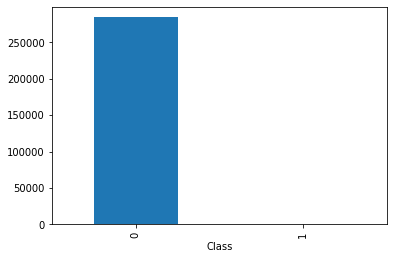
by_fraud.size().plot(kind = 'bar')<matplotlib.axes._subplots.AxesSubplot at 0x227fb41c940>
fraud['Amount'].describe()count 492.000000
mean 122.211321
std 256.683288
min 0.000000
25% 1.000000
50% 9.250000
75% 105.890000
max 2125.870000
Name: Amount, dtype: float64
normal['Amount'].describe()count 284315.000000
mean 88.291022
std 250.105092
min 0.000000
25% 5.650000
50% 22.000000
75% 77.050000
max 25691.160000
Name: Amount, dtype: float64
上面是將異常與正常的資料分開做簡單統計量呈現,我們可看出正常資料為284315筆、異常資料為492筆,大約0.9983:0.0017,此為不平衡資料,因此在這裡我們嘗試比較數個under sampling、oversampling的幾個採樣方法,並在採樣後皆使用隨機森林n=100的方法下去建模,藉此比較各種採樣方法的AIC與Accuracy。我們將使用Non sampling、under sampling、smote以及GAN with one-class classifier。而我皆保留50%原始資料當作validation set,剩餘50%則做為training set。
Non Sampling
這裡我將先以不平衡的方式直接建模,以當作其餘資料的對照組。
from sklearn.model_selection import train_test_split
fraud = df[df['Class'].isin([1])]
normal = df[df['Class'].isin([0])]

test_nor, train_nor = train_test_split(normal, test_size = 0.5)
train_fra, test_fra = train_test_split(fraud, test_size = 0.5)
data_train = pd.concat([train_nor,train_fra], axis=0)
data_test = pd.concat([test_nor,test_fra], axis=0)

train_X = data_train.iloc[:,0:30]
test_X = data_test.iloc[:,0:30]
train_y = data_train["Class"]
test_y = data_test["Class"]
forest = ensemble.RandomForestClassifier(n_estimators = 100)
forest_fit = forest.fit(train_X, train_y)
test_y_predicted = forest.predict(test_X)
accuracy_rf = metrics.accuracy_score(test_y, test_y_predicted)
print(accuracy_rf)
test_auc = metrics.roc_auc_score(test_y, test_y_predicted)
print (test_auc)ACC:0.9994803480263759
AUC:0.8678545237199384
Under Sampling
這個地方我採用下採樣方法,即從14w筆正常的訓練資料中抽出246筆與246筆異常資料的492筆資料建立分類模型。
from sklearn.model_selection import train_test_split
fraud = df[df['Class'].isin([1])]
normal = df[df['Class'].isin([0])]
test_nor, train_nor = train_test_split(normal, test_size = 0.0008652375)
train_fra, test_fra = train_test_split(fraud, test_size = 0.5)
data_train = pd.concat([train_nor,train_fra], axis=0)
data_test = pd.concat([test_nor,test_fra], axis=0) train_X = data_train.iloc[:,0:30]
test_X = data_test.iloc[:,0:30]
train_y = data_train["Class"]
test_y = data_test["Class"]from sklearn.model_selection import train_test_split
from sklearn import ensemble
from sklearn import metrics
forest = ensemble.RandomForestClassifier(n_estimators = 100)
forest_fit = forest.fit(train_X, train_y)

test_y_predicted = forest.predict(test_X)
accuracy_rf = metrics.accuracy_score(test_y, test_y_predicted)
print(accuracy_rf)


test_auc = metrics.roc_auc_score(test_y, test_y_predicted)
print (test_auc)ACC:0.9995084373222475
AUC:0.8901876266312907
SMOTE
SMOTE是很常見的採樣方法,在這裡我將使用其演算法生成用以平衡的偽資料,以進行後續分類器的訓練。
from imblearn.over_sampling import SMOTE
X_resampled, y_resampled = SMOTE().fit_resample(train_X, train_y)
X_resampled = pd.DataFrame(X_resampled)
y_resampled = pd.DataFrame(y_resampled)X_resampled.head()| 0 | 1 | 2 | 3 | 4 | 5 | 6 | 7 | 8 | 9 | … | 20 | 21 | 22 | 23 | 24 | 25 | 26 | 27 | 28 | 29 | |
|---|---|---|---|---|---|---|---|---|---|---|---|---|---|---|---|---|---|---|---|---|---|
| 0 | 142158.0 | 2.098232 | -0.120009 | -1.556132 | 0.138363 | 0.474125 | -0.357738 | 0.133597 | -0.197507 | 0.570249 | … | -0.137225 | -0.335204 | -0.897051 | 0.270364 | 0.032881 | -0.182849 | 0.206514 | -0.079001 | -0.057921 | 15.88 |
| 1 | 120533.0 | -0.231309 | -0.100840 | 0.901389 | 0.102371 | 0.193673 | 1.020901 | 0.086328 | 0.467544 | 0.523512 | … | 0.021338 | 0.160314 | 0.226446 | 0.136961 | -1.550618 | -0.454142 | -0.752112 | 0.097091 | 0.058509 | 112.78 |
| 2 | 143598.0 | 1.707347 | -2.010102 | -0.119053 | -0.621244 | -1.470343 | 1.004779 | -1.539303 | 0.351543 | 0.807437 | … | 0.417312 | 0.265302 | 0.609864 | 0.017976 | 0.337693 | -0.339032 | -0.226504 | 0.021035 | -0.009205 | 205.63 |
| 3 | 77785.0 | -0.432809 | 0.441564 | 2.135267 | 1.571277 | 0.007931 | 1.057945 | -0.090015 | 0.405717 | 0.597818 | … | 0.010397 | -0.325426 | -0.474865 | -0.051495 | -0.426681 | -0.322176 | -0.406189 | 0.233169 | 0.152133 | 7.60 |
| 4 | 37257.0 | 1.206999 | -0.933973 | 0.439600 | -0.833985 | -1.045920 | -0.002520 | -0.895569 | 0.236254 | -0.653197 | … | 0.079357 | 0.067089 | -0.156065 | 0.041761 | -0.358237 | 0.097000 | -0.379807 | 0.005337 | 0.015024 | 75.00 |
5 rows × 30 columns
forest = ensemble.RandomForestClassifier(n_estimators = 100)
forest_fit = forest.fit(X_resampled, y_resampled)

test_y_predicted = forest.predict(test_X)
accuracy_rf = metrics.accuracy_score(test_y, test_y_predicted)
print(accuracy_rf)


test_auc = metrics.roc_auc_score(test_y, test_y_predicted)
print (test_auc)
C:3-gpu-packages_launcher.py:2: DataConversionWarning: A column-vector y was passed when a 1d array was expected. Please change the shape of y to (n_samples,), for example using ravel().
ACC = 0.9994663033784401
AUC = 0.9023405417267101
ADASYN
ADASYN是另一種過採樣方法,它是Smote的改進版本。它的功能與SMOTE相同,只是稍有改進。創建這些假樣本後,它會向這些點添加一個隨機的小值,從而使其更加真實。換句話說,不是所有樣本都與原始樣本線性相關,而是它們具有更多的變異(variance),即它們是零散的。
from imblearn.over_sampling import ADASYN
X_resampled, y_resampled = ADASYN().fit_resample(train_X, train_y)
X_resampled = pd.DataFrame(X_resampled)
y_resampled = pd.DataFrame(y_resampled)
forest = ensemble.RandomForestClassifier(n_estimators = 100)
forest_fit = forest.fit(X_resampled, y_resampled)
test_y_predicted = forest.predict(test_X)
accuracy_rf = metrics.accuracy_score(test_y, test_y_predicted)
print("accuracy = %s"%accuracy_rf)
test_auc = metrics.roc_auc_score(test_y, test_y_predicted)
print ("test_auc = %d"%test_auc)C:3-gpu-packages_launcher.py:2: DataConversionWarning: A column-vector y was passed when a 1d array was expected. Please change the shape of y to (n_samples,), for example using ravel().
accuracy = 0.9993890578147933
AUC = 0.8982438459344533
GAN with One Class SVM
The generator
Set up modules
%matplotlib inline
import os
import random
import numpy as np
import pandas as pd
import matplotlib.pyplot as plt
import seaborn as sns
from tqdm import tqdm_notebook as tqdm
from keras.models import Model
from keras.layers import Input, Reshape
from keras.layers.core import Dense, Activation, Dropout, Flatten
from keras.layers.normalization import BatchNormalization
from keras.layers.convolutional import UpSampling1D, Conv1D
from keras.layers.advanced_activations import LeakyReLU
from keras.optimizers import Adam, SGD
from keras.callbacks import TensorBoard
from sklearn.preprocessing import StandardScaler

dim = 30
num = 246
g_data = f_x
Using TensorFlow backend.
Standard Scaler
ss = StandardScaler()
g_data = pd.DataFrame(ss.fit_transform(g_data))
def get_generative(G_in, dense_dim=200, out_dim= dim, lr=1e-3):
x = Dense(dense_dim)(G_in)
x = Activation('tanh')(x)
G_out = Dense(out_dim, activation='tanh')(x)
G = Model(G_in, G_out)
opt = SGD(lr=lr)
G.compile(loss='binary_crossentropy', optimizer=opt)
return G, G_out
G_in = Input(shape=[10])
G, G_out = get_generative(G_in)
G.summary()WARNING:tensorflow:From C:3-gpu-packages_backend.py:74: The name tf.get_default_graph is deprecated. Please use tf.compat.v1.get_default_graph instead.
WARNING:tensorflow:From C:3-gpu-packages_backend.py:517: The name tf.placeholder is deprecated. Please use tf.compat.v1.placeholder instead.
WARNING:tensorflow:From C:3-gpu-packages_backend.py:4138: The name tf.random_uniform is deprecated. Please use tf.random.uniform instead.
WARNING:tensorflow:From C:3-gpu-packages.py:790: The name tf.train.Optimizer is deprecated. Please use tf.compat.v1.train.Optimizer instead.
WARNING:tensorflow:From C:3-gpu-packages_backend.py:3376: The name tf.log is deprecated. Please use tf.math.log instead.
WARNING:tensorflow:From C:3-gpu-packagesimpl.py:180: add_dispatch_support.
=================================================================
input_1 (InputLayer) (None, 10) 0
_________________________________________________________________
dense_1 (Dense) (None, 200) 2200
_________________________________________________________________
activation_1 (Activation) (None, 200) 0
_________________________________________________________________
dense_2 (Dense) (None, 30) 6030
=================================================================
Total params: 8,230
Trainable params: 8,230
Non-trainable params: 0
_________________________________________________________________
建立判別器
def get_discriminative(D_in, lr=1e-3, drate=.25, n_channels= dim, conv_sz=5, leak=.2):
    x = Reshape((-1, 1))(D_in)
    x = Conv1D(n_channels, conv_sz, activation='relu')(x)
    x = Dropout(drate)(x)
    x = Flatten()(x)
    x = Dense(n_channels)(x)
    D_out = Dense(2, activation='sigmoid')(x)
    D = Model(D_in, D_out)
    dopt = Adam(lr=lr)
    D.compile(loss='binary_crossentropy', optimizer=dopt)
    return D, D_out

D_in = Input(shape=[dim])
D, D_out = get_discriminative(D_in)
D.summary()
WARNING:tensorflow:From C:3-gpu-packages_backend.py:133: The name tf.placeholder_with_default is deprecated. Please use tf.compat.v1.placeholder_with_default instead.
WARNING:tensorflow:From C:3-gpu-packagesbackend.py:3445: calling dropout (from tensorflow.python.ops.nn_ops) with keep_prob is deprecated and will be removed in a future version.
Instructions for updating:
Please use rate instead of keep_prob. Rate should be set to rate = 1 - keep_prob.
________________________________________________________________
Layer (type) Output Shape Param #
=================================================================
input_2 (InputLayer) (None, 30) 0
_________________________________________________________________
reshape_1 (Reshape) (None, 30, 1) 0
_________________________________________________________________
conv1d_1 (Conv1D) (None, 26, 30) 180
_________________________________________________________________
dropout_1 (Dropout) (None, 26, 30) 0
_________________________________________________________________
flatten_1 (Flatten) (None, 780) 0
_________________________________________________________________
dense_3 (Dense) (None, 30) 23430
_________________________________________________________________
dense_4 (Dense) (None, 2) 62
=================================================================
Total params: 23,672
Trainable params: 23,672
Non-trainable params: 0
_________________________________________________________________
串接兩神經網路
def set_trainability(model, trainable=False):
    model.trainable = trainable
    for layer in model.layers:
        layer.trainable = trainable

def make_gan(GAN_in, G, D):
    set_trainability(D, False)
    x = G(GAN_in)
    GAN_out = D(x)
    GAN = Model(GAN_in, GAN_out)
    GAN.compile(loss='binary_crossentropy', optimizer=G.optimizer)
    return GAN, GAN_out

GAN_in = Input([10])
GAN, GAN_out = make_gan(GAN_in, G, D)
GAN.summary()
Layer (type) Output Shape Param #
=================================================================
input_3 (InputLayer) (None, 10) 0
_________________________________________________________________
model_1 (Model) (None, 30) 8230
_________________________________________________________________
model_2 (Model) (None, 2) 23672
=================================================================
Total params: 31,902
Trainable params: 8,230
Non-trainable params: 23,672
_________________________________________________________________
def sample_data_and_gen(G, noise_dim=10, n_samples= num):
    XT = np.array(g_data)
    XN_noise = np.random.uniform(0, 1, size=[n_samples, noise_dim])
    XN = G.predict(XN_noise)
    X = np.concatenate((XT, XN))
    y = np.zeros((2*n_samples, 2))
    y[:n_samples, 1] = 1
    y[n_samples:, 0] = 1
    return X, y

def pretrain(G, D, noise_dim=10, n_samples = num, batch_size=32):
    X, y = sample_data_and_gen(G, n_samples=n_samples, noise_dim=noise_dim)
    set_trainability(D, True)
    D.fit(X, y, epochs=1, batch_size=batch_size)

pretrain(G, D)

def sample_noise(G, noise_dim=10, n_samples=num):
    X = np.random.uniform(0, 1, size=[n_samples, noise_dim])
    y = np.zeros((n_samples, 2))
    y[:, 1] = 1
    return X, y
Epoch 1/1 492/492 [==============================] - ETA: 7s - loss: 0.662 - 1s 1ms/step - loss: 0.4410
訓練生成對抗網路
訓練生成對抗網路,並存取最後一次生成器產生結果
def train(GAN, G, D, epochs=100, n_samples= num, noise_dim=10, batch_size=32, verbose=False, v_freq=dim,):
    d_loss = []
    g_loss = []
    e_range = range(epochs)
    if verbose:
        e_range = tqdm(e_range)
    for epoch in e_range:
        X, y = sample_data_and_gen(G, n_samples=n_samples, noise_dim=noise_dim)
        set_trainability(D, True)
        d_loss.append(D.train_on_batch(X, y))
        xx,yy = X,y

        X, y = sample_noise(G, n_samples=n_samples, noise_dim=noise_dim)
        set_trainability(D, False)
        g_loss.append(GAN.train_on_batch(X, y))
        if verbose and (epoch + 1) % v_freq == 0:
            print("Epoch #{}: Generative Loss: {}, Discriminative Loss: {}".format(epoch + 1, g_loss[-1], d_loss[-1]))
    return d_loss, g_loss, xx, yy

d_loss, g_loss ,xx,yy= train(GAN, G, D, verbose=True)
HBox(children=(IntProgress(value=0), HTML(value=’’)))
Epoch #30: Generative Loss: 4.016930103302002, Discriminative Loss: 0.05247233808040619 Epoch #60: Generative Loss: 4.552446365356445, Discriminative Loss: 0.03850032016634941 Epoch #90: Generative Loss: 4.267617702484131, Discriminative Loss: 0.12488271296024323
自動化echo
損失函數
ax = pd.DataFrame(
    {
        'Generative Loss': g_loss,
        'Discriminative Loss': d_loss,
    }
).plot(title='Training loss', logy=True)
ax.set_xlabel("Epochs")
ax.set_ylabel("Loss")
Text(0, 0.5, ‘Loss’)

png
new_data = xx[num:num*2+1]
#pd.DataFrame(new_data)
#pd.DataFrame(ss.inverse_transform(xx[0:492]))
#pd.DataFrame(ss.inverse_transform(xx))One Class Learning
one class svm
from sklearn import svm

clf = svm.OneClassSVM(kernel='rbf', gamma='auto').fit(xx[0:246])

origin = pd.DataFrame(clf.score_samples(xx[0:246]))
origin.describe()| 0 | |
|---|---|
| count | 246.000000 |
| mean | 23.916780 |
| std | 6.798673 |
| min | 1.089954 |
| 25% | 20.998108 |
| 50% | 25.390590 |
| 75% | 28.886752 |
| max | 33.391387 |
new = pd.DataFrame(clf.score_samples(xx[246:493]))
new.describe()| 0 | |
|---|---|
| count | 246.000000 |
| mean | 29.028060 |
| std | 1.533237 |
| min | 25.520972 |
| 25% | 27.996268 |
| 50% | 28.910111 |
| 75% | 30.022437 |
| max | 33.144183 |
occ = pd.concat([pd.DataFrame(new[0] < origin[0].min()),pd.DataFrame(new[0] > origin[0].max())], axis=1)
occ['ava'] = pd.DataFrame(occ.iloc[:,1:2] == occ.iloc[:,0:1])
occ| 0 | 0 | ava | |
|---|---|---|---|
| 0 | False | False | True |
| 1 | False | False | True |
| 2 | False | False | True |
| 3 | False | False | True |
| 4 | False | False | True |
| 5 | False | False | True |
| 6 | False | False | True |
| 7 | False | False | True |
| 8 | False | False | True |
| 9 | False | False | True |
| 10 | False | False | True |
| 11 | False | False | True |
| 12 | False | False | True |
| 13 | False | False | True |
| 14 | False | False | True |
| 15 | False | False | True |
| 16 | False | False | True |
| 17 | False | False | True |
| 18 | False | False | True |
| 19 | False | False | True |
| 20 | False | False | True |
| 21 | False | False | True |
| 22 | False | False | True |
| 23 | False | False | True |
| 24 | False | False | True |
| 25 | False | False | True |
| 26 | False | False | True |
| 27 | False | False | True |
| 28 | False | False | True |
| 29 | False | False | True |
| … | … | … | … |
| 216 | False | False | True |
| 217 | False | False | True |
| 218 | False | False | True |
| 219 | False | False | True |
| 220 | False | False | True |
| 221 | False | False | True |
| 222 | False | False | True |
| 223 | False | False | True |
| 224 | False | False | True |
| 225 | False | False | True |
| 226 | False | False | True |
| 227 | False | False | True |
| 228 | False | False | True |
| 229 | False | False | True |
| 230 | False | False | True |
| 231 | False | False | True |
| 232 | False | False | True |
| 233 | False | False | True |
| 234 | False | False | True |
| 235 | False | False | True |
| 236 | False | False | True |
| 237 | False | False | True |
| 238 | False | False | True |
| 239 | False | False | True |
| 240 | False | False | True |
| 241 | False | False | True |
| 242 | False | False | True |
| 243 | False | False | True |
| 244 | False | False | True |
| 245 | False | False | True |
246 rows × 3 columns
err = sum(occ['ava'] == False)/len(occ['ava'])
err
0.0
合併資料
re = 577
new_data = pd.DataFrame(xx[246:493])
new_data.columns = g_data.columns
data = pd.concat([g_data,new_data], axis=0)
for i in range(re):
    d_loss, g_loss ,x1,yy= train(GAN, G, D, epochs=1,verbose=True)
    new_data = pd.DataFrame(ss.inverse_transform(xx[246:493]))
    data = pd.concat([data,new_data], axis=0)

data['sum'] = 1
HBox(children=(IntProgress(value=0, max=1), HTML(value=’’)))
資料分析
合併新舊資料
data.columns = df.columns
data = pd.concat([data_train,data], axis=0)
建構簡易分類器
from sklearn.model_selection import train_test_split
from sklearn import ensemble
from sklearn import metrics

train_X = data.iloc[:,0:30]
test_X = data_test.iloc[:,0:30]
train_y = data["Class"]
test_y = data_test["Class"]


forest = ensemble.RandomForestClassifier(n_estimators = 100)
forest_fit = forest.fit(train_X, train_y)

test_y_predicted = forest.predict(test_X)
accuracy_rf = metrics.accuracy_score(test_y, test_y_predicted)
print(accuracy_rf)


test_auc = metrics.roc_auc_score(test_y, test_y_predicted)
print (test_auc)
ACC = 0.999557596696722
AUC = 0.9003572630796582
Results
將各採樣方法的結果建立表格並畫出
result <- data.frame()
result = data.frame(c(0.9994803480263759,0.8678545237199384))
result$Under_Sampling = data.frame(c(0.9995084373222475,0.8901876266312907))
result$SMOTE = data.frame(c(0.9994663033784401,0.9023405417267101))
result$ADASYN = data.frame(c(0.9993890578147933,0.8982438459344533))
result$GAN = data.frame(c(0.999557596696722,0.9003572630796582))
colnames(result) <- c("Non Sampling","Under Sampling","SMOTE","ADASYN","GAN")
rownames(result) <- c("ACC","AUC")
#result$index <- c("ACC","AUC")
result  = data.frame(t(result))
result
## ACC AUC
## Non Sampling 0.9994803 0.8678545
## Under Sampling 0.9995084 0.8901876
## SMOTE 0.9994663 0.9023405
## ADASYN 0.9993891 0.8982438
## GAN 0.9995576 0.9003573library(ggplot2)
ggplot(data = result)+
geom_point(mapping = aes(x = ACC,y = AUC,color = rownames(result)),size=7)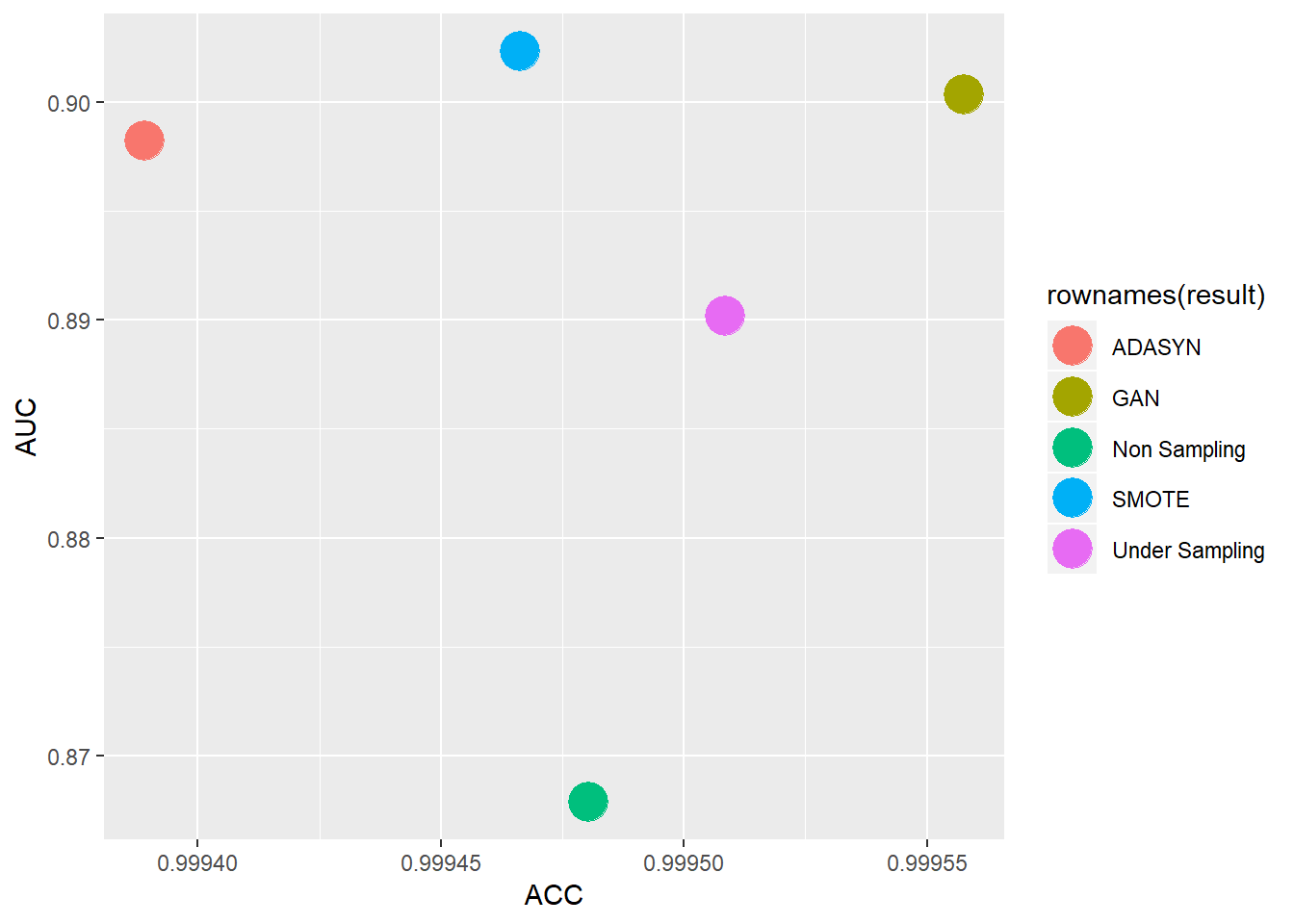 從上表可看出,若單考量AUC的情況下,SMOTE有較佳的結果、GAN則排在第二,若是以綜合考量的情況下(落於右上角的),則是GAN的結果較佳,從此表可看出,SMOTE與我的One class-GAN在AUC有差不多的結果,而單就運算成本來說GAN則遠遠高出不少,但在資料不大的情況下(像此例),則可以交叉多種採樣方法來使用,後續可能會使用其他種方法或是資料來比較GAN與其他採樣方法的效果,畢竟還是希望GAN在資料過採樣上能有較好的表現。