這次我將使用先前東海大學大數據競賽的初賽資料,也就是熱成化加工的數據資料,而該資料中一共有8類,我將資料的第5與8類挑選出來,並僅取3筆第5類資料與136筆第8類資料作為訓練資料,而驗證資料則為9筆第5類資料與136筆第8類資料作為測試資料,因此我們的目標是使用生成對抗網路來生成第5類資料以達到資料平衡後進行後續的分類分析。
1.準備資料
1.1 讀取資料
import pandas as pd
import numpy as np

df = pd.read_csv('C:/Users/User/OneDrive - student.nsysu.edu.tw/Educations/Contests/thu_bigdata/初賽/train model/train.csv')
df.head()| V1 | V2 | V3 | V4 | V5 | V6 | V7 | V8 | V9 | V10 | … | V441 | V442 | V443 | V444 | V445 | V446 | V447 | V448 | V449 | y | |
|---|---|---|---|---|---|---|---|---|---|---|---|---|---|---|---|---|---|---|---|---|---|
| 0 | 65.9 | 65.9 | 65.9 | 65.9 | 66.6 | 68.0 | 69.4 | 71.7 | 74.3 | 77.1 | … | 0.0 | 0.0 | 0.0 | 0.0 | 0.0 | 0.0 | 0.0 | 0.0 | 0.0 | 1 |
| 1 | 65.8 | 65.8 | 65.8 | 65.8 | 67.2 | 68.9 | 70.8 | 73.6 | 76.9 | 80.0 | … | 0.0 | 0.0 | 0.0 | 0.0 | 0.0 | 0.0 | 0.0 | 0.0 | 0.0 | 1 |
| 2 | 64.2 | 64.2 | 64.2 | 64.2 | 65.7 | 67.5 | 69.6 | 72.3 | 75.1 | 78.4 | … | 0.0 | 0.0 | 0.0 | 0.0 | 0.0 | 0.0 | 0.0 | 0.0 | 0.0 | 1 |
| 3 | 64.9 | 64.9 | 64.9 | 64.9 | 65.6 | 66.4 | 67.1 | 68.3 | 69.6 | 70.9 | … | 0.0 | 0.0 | 0.0 | 0.0 | 0.0 | 0.0 | 0.0 | 0.0 | 0.0 | 1 |
| 4 | 66.0 | 66.0 | 66.0 | 66.0 | 67.3 | 68.6 | 70.0 | 72.0 | 74.0 | 76.4 | … | 0.0 | 0.0 | 0.0 | 0.0 | 0.0 | 0.0 | 0.0 | 0.0 | 0.0 | 1 |
5 rows x 450 columns
from sklearn.model_selection import train_test_split
data1 = df[df['y'].isin([5])].iloc[0:3,:]
data2 = df[df['y'].isin([8])]
train_nor = data1
test_nor = df[df['y'].isin([5])].iloc[5:14,:]
train_fra, test_fra = train_test_split(data2, test_size = 0.5)
data_train = pd.concat([train_nor,train_fra], axis=0)
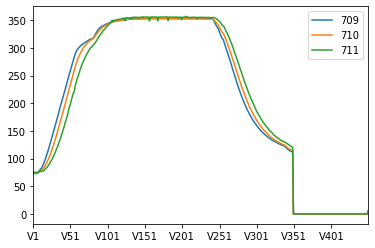
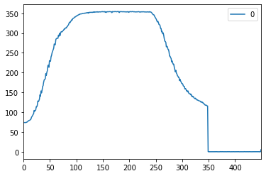
data_test = pd.concat([test_nor,test_fra], axis=0)pd.DataFrame(np.transpose(data1)).plot()
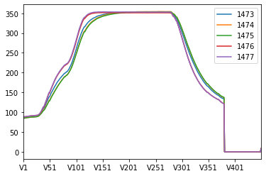
pd.DataFrame(np.transpose(data2.head())).plot()<matplotlib.axes._subplots.AxesSubplot at 0x168ba4d4710>
1.2 Non Sampling
先嘗試使用不採樣的方式建模型,觀察直接做分類的效果。
from sklearn import ensemble
from sklearn import metrics

train_X = data_train.iloc[:,0:449]
test_X = data_test.iloc[:,0:449]
train_y = data_train["y"]
test_y = data_test["y"]

forest = ensemble.RandomForestClassifier(n_estimators = 100)
forest_fit = forest.fit(train_X, train_y)

test_y_predicted = forest.predict(test_X)
accuracy_rf = metrics.accuracy_score(test_y, test_y_predicted)
print(accuracy_rf)

test_auc = metrics.roc_auc_score(test_y, test_y_predicted)
print (test_auc)
0.993103448275862 0.9444444444444444
可以發現auc高達:0.944,因此這筆資料可能特徵太過容易做分類,因此後續的平衡資料分析可能效果不會太過顯著。
2. GAN with one class svm
2.1 建立GAN
# import modules
%matplotlib inline
import os
import random
import numpy as np
import pandas as pd
import matplotlib.pyplot as plt
import seaborn as sns
from tqdm import tqdm_notebook as tqdm
from keras.models import Model
from keras.layers import Input, Reshape
from keras.layers.core import Dense, Activation, Dropout, Flatten
from keras.layers.normalization import BatchNormalization
from keras.layers.convolutional import UpSampling1D, Conv1D
from keras.layers.advanced_activations import LeakyReLU
from keras.optimizers import Adam, SGD
from keras.callbacks import TensorBoard
from sklearn.preprocessing import StandardScaler

# set parameters
dim = 450
num = 3
g_data = data1

# Standard Scaler
ss = StandardScaler()
g_data = pd.DataFrame(ss.fit_transform(g_data))


# generator
def get_generative(G_in, dense_dim=200, out_dim= dim, lr=1e-3):
    x = Dense(dense_dim)(G_in)
    x = Activation('tanh')(x)
    G_out = Dense(out_dim, activation='tanh')(x)
    G = Model(G_in, G_out)
    opt = SGD(lr=lr)
    G.compile(loss='binary_crossentropy', optimizer=opt)
    return G, G_out

G_in = Input(shape=[10])
G, G_out = get_generative(G_in)
G.summary()

# discriminator
def get_discriminative(D_in, lr=1e-3, drate=.25, n_channels= dim, conv_sz=5, leak=.2):
    x = Reshape((-1, 1))(D_in)
    x = Conv1D(n_channels, conv_sz, activation='relu')(x)
    x = Dropout(drate)(x)
    x = Flatten()(x)
    x = Dense(n_channels)(x)
    D_out = Dense(2, activation='sigmoid')(x)
    D = Model(D_in, D_out)
    dopt = Adam(lr=lr)
    D.compile(loss='binary_crossentropy', optimizer=dopt)
    return D, D_out

D_in = Input(shape=[dim])
D, D_out = get_discriminative(D_in)
D.summary()

# set up gan
def set_trainability(model, trainable=False):
    model.trainable = trainable
    for layer in model.layers:
        layer.trainable = trainable

def make_gan(GAN_in, G, D):
    set_trainability(D, False)
    x = G(GAN_in)
    GAN_out = D(x)
    GAN = Model(GAN_in, GAN_out)
    GAN.compile(loss='binary_crossentropy', optimizer=G.optimizer)
    return GAN, GAN_out

GAN_in = Input([10])
GAN, GAN_out = make_gan(GAN_in, G, D)
GAN.summary()

# pre train
def sample_data_and_gen(G, noise_dim=10, n_samples= num):
    XT = np.array(g_data)
    XN_noise = np.random.uniform(0, 1, size=[n_samples, noise_dim])
    XN = G.predict(XN_noise)
    X = np.concatenate((XT, XN))
    y = np.zeros((2*n_samples, 2))
    y[:n_samples, 1] = 1
    y[n_samples:, 0] = 1
    return X, y

def pretrain(G, D, noise_dim=10, n_samples = num, batch_size=32):
    X, y = sample_data_and_gen(G, n_samples=n_samples, noise_dim=noise_dim)
    set_trainability(D, True)
    D.fit(X, y, epochs=1, batch_size=batch_size)

pretrain(G, D)

def sample_noise(G, noise_dim=10, n_samples=num):
    X = np.random.uniform(0, 1, size=[n_samples, noise_dim])
    y = np.zeros((n_samples, 2))
    y[:, 1] = 1
    return X, y
Using TensorFlow backend.
WARNING:tensorflow:From C:3-gpu-packages_backend.py:74: The name tf.get_default_graph is deprecated. Please use tf.compat.v1.get_default_graph instead.
WARNING:tensorflow:From C:3-gpu-packages_backend.py:517: The name tf.placeholder is deprecated. Please use tf.compat.v1.placeholder instead.
WARNING:tensorflow:From C:3-gpu-packages_backend.py:4138: The name tf.random_uniform is deprecated. Please use tf.random.uniform instead.
WARNING:tensorflow:From C:3-gpu-packages.py:790: The name tf.train.Optimizer is deprecated. Please use tf.compat.v1.train.Optimizer instead.
WARNING:tensorflow:From C:3-gpu-packages_backend.py:3376: The name tf.log is deprecated. Please use tf.math.log instead.
WARNING:tensorflow:From C:3-gpu-packagesimpl.py:180: add_dispatch_support.
=================================================================
input_1 (InputLayer) (None, 10) 0
_________________________________________________________________
dense_1 (Dense) (None, 200) 2200
_________________________________________________________________
activation_1 (Activation) (None, 200) 0
_________________________________________________________________
dense_2 (Dense) (None, 450) 90450
=================================================================
Total params: 92,650
Trainable params: 92,650
Non-trainable params: 0
_________________________________________________________________
WARNING:tensorflow:From C:3-gpu-packages_backend.py:133: The name tf.placeholder_with_default is deprecated. Please use tf.compat.v1.placeholder_with_default instead.
WARNING:tensorflow:From C:3-gpu-packagesbackend.py:3445: calling dropout (from tensorflow.python.ops.nn_ops) with keep_prob is deprecated and will be removed in a future version.
Instructions for updating:
Please use rate instead of keep_prob. Rate should be set to rate = 1 - keep_prob.
________________________________________________________________
Layer (type) Output Shape Param #
=================================================================
input_2 (InputLayer) (None, 450) 0
_________________________________________________________________
reshape_1 (Reshape) (None, 450, 1) 0
_________________________________________________________________
conv1d_1 (Conv1D) (None, 446, 450) 2700
_________________________________________________________________
dropout_1 (Dropout) (None, 446, 450) 0
_________________________________________________________________
flatten_1 (Flatten) (None, 200700) 0
_________________________________________________________________
dense_3 (Dense) (None, 450) 90315450
_________________________________________________________________
dense_4 (Dense) (None, 2) 902
=================================================================
Total params: 90,319,052
Trainable params: 90,319,052
Non-trainable params: 0
_________________________________________________________________
_________________________________________________________________
Layer (type) Output Shape Param #
=================================================================
input_3 (InputLayer) (None, 10) 0
_________________________________________________________________
model_1 (Model) (None, 450) 92650
_________________________________________________________________
model_2 (Model) (None, 2) 90319052
=================================================================
Total params: 90,411,702
Trainable params: 92,650
Non-trainable params: 90,319,052
_________________________________________________________________
Epoch 1/1
6/6 [==============================] - 2s 342ms/step - loss: 0.6915
2.2 訓練GAN
# training
def train(GAN, G, D, epochs=300, n_samples= num, noise_dim=10, batch_size=32, verbose=False, v_freq=dim,):
    d_loss = []
    g_loss = []
    e_range = range(epochs)
    if verbose:
        e_range = tqdm(e_range)
    for epoch in e_range:
        X, y = sample_data_and_gen(G, n_samples=n_samples, noise_dim=noise_dim)
        set_trainability(D, True)
        d_loss.append(D.train_on_batch(X, y))
        xx,yy = X,y

        X, y = sample_noise(G, n_samples=n_samples, noise_dim=noise_dim)
        set_trainability(D, False)
        g_loss.append(GAN.train_on_batch(X, y))
        if verbose and (epoch + 1) % v_freq == 0:
            print("Epoch #{}: Generative Loss: {}, Discriminative Loss: {}".format(epoch + 1, g_loss[-1], d_loss[-1]))
    return d_loss, g_loss, xx, yy

d_loss, g_loss ,xx,yy= train(GAN, G, D, verbose=True)
HBox(children=(IntProgress(value=0, max=1), HTML(value=’’)))
2.3 One Class SVM
將標準化後的原始資料建立一個One Class SVM
from sklearn import svm

clf = svm.OneClassSVM(kernel='linear', gamma='auto').fit(xx[0:3])
origin = pd.DataFrame(clf.score_samples(xx[0:3]))
origin.describe()| 0 | |
|---|---|
| count | 3.000000e+00 |
| mean | -8.052818e-14 |
| std | 1.144001e-06 |
| min | -8.919722e-07 |
| 25% | -6.449020e-07 |
| 50% | -3.978317e-07 |
| 75% | 4.459860e-07 |
| max | 1.289804e-06 |
使用生成資料計算它們的score
new = pd.DataFrame(clf.score_samples(xx[3:6]))
new.describe()| 0 | |
|---|---|
| count | 3.000000e+00 |
| mean | 3.488132e-09 |
| std | 3.022134e-09 |
| min | 5.208247e-10 |
| 25% | 1.951068e-09 |
| 50% | 3.381310e-09 |
| 75% | 4.971785e-09 |
| max | 6.562260e-09 |
occ = pd.concat([pd.DataFrame(new[0] < origin[0].min()),pd.DataFrame(new[0] > origin[0].max())], axis=1)
occ['ava'] = pd.DataFrame(occ.iloc[:,1:2] == occ.iloc[:,0:1])
occ| 0 | 0 | ava | |
|---|---|---|---|
| 0 | False | False | True |
| 1 | False | False | True |
| 2 | False | False | True |
2.4 計算生成異常率
err = sum(occ['ava'] == False)/len(occ['ava'])
err
0.0
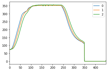
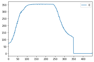
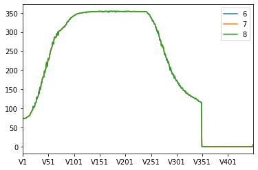
畫出生成的資料圖,第一張圖片為原始3張資料,下三張資料則為迭代後所生成的資料,基本肉眼難以分辨真偽。
pd.DataFrame(np.transpose(pd.DataFrame(ss.inverse_transform(xx[0:3])))).plot()
pd.DataFrame(np.transpose(pd.DataFrame(ss.inverse_transform(xx[3:4])))).plot()
pd.DataFrame(np.transpose(pd.DataFrame(ss.inverse_transform(xx[4:5])))).plot()
pd.DataFrame(np.transpose(data_train1.iloc[6:9,:])).plot()
<matplotlib.axes._subplots.AxesSubplot at 0x169afe20748>
3. Balance and Validate
3.1 Balance data
生成符合標準的資料並合併舊有資料,以產生平衡的訓練資料。這裡我們生成45次*3的第5類樣本,並與舊的訓練資料做合併。
# balance train data
re = 45
new_data = pd.DataFrame(xx[3:6])
new_data.columns = g_data.columns
data = pd.concat([g_data,new_data], axis=0)
for i in range(re):
    d_loss, g_loss ,xx,yy= train(GAN, G, D, verbose=True)
    new_data = pd.DataFrame((xx[3:6]))
    data = pd.concat([data,new_data], axis=0)
# anti Scaler
data_train1 = pd.DataFrame(ss.inverse_transform(data))
data_train1 = data_train1.iloc[:,0:449]
data_train1['y'] = 5
data_train1.head()| 0 | 1 | 2 | 3 | 4 | 5 | 6 | 7 | 8 | 9 | … | 440 | 441 | 442 | 443 | 444 | 445 | 446 | 447 | 448 | y | |
|---|---|---|---|---|---|---|---|---|---|---|---|---|---|---|---|---|---|---|---|---|---|
| 0 | 72.800000 | 72.800000 | 72.800000 | 72.800000 | 73.200000 | 73.900000 | 75.000000 | 76.200000 | 77.700000 | 79.500000 | … | 0.000000 | 0.000000 | 0.000000 | 0.000000 | 0.000000 | 0.000000 | 0.000000 | 0.000000 | 0.000000 | 5 |
| 1 | 73.400000 | 73.400000 | 73.400000 | 73.400000 | 73.700000 | 74.100000 | 74.700000 | 75.100000 | 75.900000 | 77.000000 | … | 0.000000 | 0.000000 | 0.000000 | 0.000000 | 0.000000 | 0.000000 | 0.000000 | 0.000000 | 0.000000 | 5 |
| 2 | 75.400000 | 75.400000 | 75.400000 | 75.400000 | 74.000000 | 75.300000 | 73.600000 | 75.700000 | 76.400000 | 76.300000 | … | 0.000000 | 0.000000 | 0.000000 | 0.000000 | 0.000000 | 0.000000 | 0.000000 | 0.000000 | 0.000000 | 5 |
| 3 | 73.878938 | 73.787891 | 73.843798 | 73.806621 | 73.749946 | 74.432668 | 74.472183 | 75.593569 | 76.449077 | 77.687163 | … | -0.029956 | 0.083634 | -0.076972 | 0.121764 | -0.076075 | -0.037339 | -0.177477 | -0.117038 | -0.112122 | 5 |
| 4 | 73.853302 | 73.748743 | 73.832179 | 73.800596 | 73.730168 | 74.408377 | 74.383461 | 75.584100 | 76.527027 | 77.752469 | … | 0.055286 | 0.058407 | -0.067959 | 0.057132 | -0.031436 | 0.031824 | -0.173006 | -0.083470 | -0.011171 | 5 |
5 rows ?? 450 columns
data_train1.columns = df.columns

data_train1 = pd.concat([data_train1,train_fra], axis=0)
data_train1| V1 | V2 | V3 | V4 | V5 | V6 | V7 | V8 | V9 | V10 | … | V441 | V442 | V443 | V444 | V445 | V446 | V447 | V448 | V449 | y | |
|---|---|---|---|---|---|---|---|---|---|---|---|---|---|---|---|---|---|---|---|---|---|
| 0 | 72.800000 | 72.800000 | 72.800000 | 72.800000 | 73.200000 | 73.900000 | 75.000000 | 76.200000 | 77.700000 | 79.500000 | … | 0.000000 | 0.000000 | 0.000000 | 0.000000 | 0.000000 | 0.000000 | 0.000000 | 0.000000 | 0.000000 | 5 |
| 1 | 73.400000 | 73.400000 | 73.400000 | 73.400000 | 73.700000 | 74.100000 | 74.700000 | 75.100000 | 75.900000 | 77.000000 | … | 0.000000 | 0.000000 | 0.000000 | 0.000000 | 0.000000 | 0.000000 | 0.000000 | 0.000000 | 0.000000 | 5 |
| 2 | 75.400000 | 75.400000 | 75.400000 | 75.400000 | 74.000000 | 75.300000 | 73.600000 | 75.700000 | 76.400000 | 76.300000 | … | 0.000000 | 0.000000 | 0.000000 | 0.000000 | 0.000000 | 0.000000 | 0.000000 | 0.000000 | 0.000000 | 5 |
| 3 | 73.878938 | 73.787891 | 73.843798 | 73.806621 | 73.749946 | 74.432668 | 74.472183 | 75.593569 | 76.449077 | 77.687163 | … | -0.029956 | 0.083634 | -0.076972 | 0.121764 | -0.076075 | -0.037339 | -0.177477 | -0.117038 | -0.112122 | 5 |
| 4 | 73.853302 | 73.748743 | 73.832179 | 73.800596 | 73.730168 | 74.408377 | 74.383461 | 75.584100 | 76.527027 | 77.752469 | … | 0.055286 | 0.058407 | -0.067959 | 0.057132 | -0.031436 | 0.031824 | -0.173006 | -0.083470 | -0.011171 | 5 |
| 5 | 74.033387 | 73.828074 | 73.997849 | 73.827376 | 73.745855 | 74.546560 | 74.443570 | 75.625994 | 76.468237 | 77.657693 | … | -0.006352 | 0.039396 | -0.196884 | -0.117058 | 0.136729 | 0.017175 | -0.251505 | -0.132704 | -0.105839 | 5 |
| 6 | 73.838466 | 73.865908 | 73.932729 | 73.813165 | 73.772236 | 74.401260 | 74.430234 | 75.597535 | 76.489400 | 77.574342 | … | -0.034173 | 0.088334 | -0.064008 | 0.193388 | -0.090340 | -0.023506 | -0.206758 | 0.067784 | 0.069030 | 5 |
| 7 | 73.968721 | 73.812409 | 73.857895 | 73.717200 | 73.693565 | 74.388412 | 74.394390 | 75.600145 | 76.585469 | 77.710865 | … | 0.114202 | -0.015879 | -0.125624 | 0.023347 | 0.107551 | 0.048280 | -0.147636 | -0.103668 | -0.138246 | 5 |
| 8 | 73.908992 | 73.781621 | 73.926368 | 73.766520 | 73.760308 | 74.445831 | 74.446917 | 75.606023 | 76.497831 | 77.589515 | … | -0.041476 | 0.056263 | -0.066880 | 0.172397 | -0.033083 | 0.051897 | -0.224216 | -0.025964 | -0.027097 | 5 |
| 9 | 73.833207 | 73.783907 | 73.892912 | 73.854442 | 73.729920 | 74.470831 | 74.365985 | 75.597333 | 76.568559 | 77.582685 | … | -0.102751 | -0.029668 | -0.064789 | 0.049890 | -0.004794 | 0.149417 | -0.260081 | -0.116775 | 0.111941 | 5 |
| 10 | 73.994793 | 73.965737 | 73.925414 | 73.808158 | 73.731936 | 74.435733 | 74.394966 | 75.592090 | 76.549678 | 77.688691 | … | 0.128079 | 0.010344 | -0.145365 | -0.082035 | 0.094352 | -0.022679 | -0.159005 | -0.012578 | -0.019866 | 5 |
| 11 | 73.921052 | 73.742424 | 73.917943 | 73.831390 | 73.779571 | 74.519111 | 74.425761 | 75.595641 | 76.445714 | 77.748555 | … | 0.074233 | 0.072568 | -0.100333 | 0.028147 | -0.028838 | 0.012675 | -0.244881 | -0.043691 | -0.055285 | 5 |
| 12 | 73.945725 | 74.022831 | 73.799910 | 73.811668 | 73.704601 | 74.410911 | 74.419966 | 75.552058 | 76.590904 | 77.630128 | … | 0.134087 | -0.084532 | -0.049599 | 0.057422 | -0.044590 | 0.045514 | -0.119169 | -0.014131 | -0.030355 | 5 |
| 13 | 73.847404 | 73.851404 | 73.834936 | 73.837091 | 73.752652 | 74.407529 | 74.403361 | 75.593328 | 76.518159 | 77.734077 | … | 0.097375 | 0.055233 | -0.066815 | 0.075503 | -0.075143 | -0.041789 | -0.159652 | 0.005027 | -0.005929 | 5 |
| 14 | 73.947727 | 73.815542 | 73.778450 | 73.817962 | 73.746453 | 74.486696 | 74.442733 | 75.579440 | 76.511518 | 77.779590 | … | 0.074677 | 0.022892 | -0.038355 | -0.022592 | -0.042554 | 0.031449 | -0.138216 | -0.142730 | -0.080931 | 5 |
| 15 | 73.925566 | 73.882039 | 73.803870 | 73.755239 | 73.737663 | 74.392020 | 74.484533 | 75.546649 | 76.469431 | 77.668451 | … | 0.056594 | 0.033979 | -0.038682 | 0.179853 | -0.102456 | -0.024040 | -0.120280 | -0.075957 | -0.132942 | 5 |
| 16 | 73.879871 | 73.832736 | 73.765226 | 73.842119 | 73.678049 | 74.442019 | 74.425773 | 75.551428 | 76.550654 | 77.653180 | … | -0.033763 | -0.001817 | -0.019532 | 0.071347 | -0.097678 | 0.130779 | -0.145152 | -0.150288 | 0.008012 | 5 |
| 17 | 73.919003 | 73.947922 | 73.914270 | 73.758956 | 73.694773 | 74.369162 | 74.410338 | 75.610844 | 76.628720 | 77.475921 | … | -0.026706 | -0.047545 | -0.084694 | 0.167542 | 0.031129 | 0.087049 | -0.178141 | 0.022013 | 0.016506 | 5 |
| 18 | 73.971674 | 73.763293 | 74.020434 | 73.724856 | 73.762588 | 74.452660 | 74.403516 | 75.655780 | 76.551840 | 77.599423 | … | 0.053126 | 0.033941 | -0.144173 | 0.108152 | 0.113208 | 0.053927 | -0.259089 | 0.046648 | -0.059140 | 5 |
| 19 | 73.873470 | 73.814242 | 73.904509 | 73.856897 | 73.749162 | 74.465535 | 74.375105 | 75.619237 | 76.534312 | 77.680803 | … | -0.042148 | 0.013516 | -0.122904 | -0.069041 | 0.063800 | 0.022003 | -0.226773 | -0.142803 | 0.034888 | 5 |
| 20 | 73.969568 | 73.822431 | 74.036429 | 73.735112 | 73.774298 | 74.440964 | 74.397474 | 75.639241 | 76.548028 | 77.586242 | … | 0.087750 | 0.043553 | -0.130206 | 0.125775 | 0.083214 | 0.035035 | -0.249830 | 0.123683 | -0.000971 | 5 |
| 21 | 73.927520 | 74.056388 | 73.844742 | 73.861624 | 73.705676 | 74.421972 | 74.473550 | 75.569122 | 76.514698 | 77.557719 | … | 0.000086 | -0.033800 | -0.100008 | 0.070435 | -0.060626 | -0.034627 | -0.141316 | -0.062197 | -0.067468 | 5 |
| 22 | 73.984382 | 73.757923 | 74.022921 | 73.717943 | 73.752087 | 74.444237 | 74.422848 | 75.641828 | 76.514564 | 77.630938 | … | 0.108226 | 0.069669 | -0.160519 | 0.136394 | 0.088176 | 0.021186 | -0.245913 | 0.076903 | -0.121950 | 5 |
| 23 | 73.844933 | 73.775766 | 73.813972 | 73.798765 | 73.712739 | 74.374528 | 74.440031 | 75.579750 | 76.483491 | 77.740687 | … | 0.082464 | 0.126852 | -0.060992 | 0.167039 | -0.126541 | -0.030765 | -0.131213 | -0.005674 | -0.090124 | 5 |
| 24 | 73.916875 | 73.933067 | 73.947333 | 73.832679 | 73.732364 | 74.427197 | 74.387339 | 75.593724 | 76.540152 | 77.620734 | … | 0.075887 | 0.012468 | -0.133915 | 0.024909 | 0.029358 | 0.004349 | -0.205712 | 0.034473 | 0.027344 | 5 |
| 25 | 74.030343 | 74.039697 | 73.894679 | 73.742541 | 73.733480 | 74.385694 | 74.423811 | 75.570987 | 76.566650 | 77.622330 | … | 0.060378 | -0.029324 | -0.112027 | -0.050489 | 0.119597 | -0.032428 | -0.108609 | -0.083925 | -0.028786 | 5 |
| 26 | 73.956202 | 73.927742 | 73.750810 | 73.843393 | 73.650193 | 74.452178 | 74.444872 | 75.543567 | 76.546764 | 77.663028 | … | -0.030830 | -0.075546 | -0.087859 | -0.067736 | 0.008812 | 0.088911 | -0.113084 | -0.282765 | -0.099524 | 5 |
| 27 | 73.918950 | 73.873934 | 73.866887 | 73.870729 | 73.751639 | 74.505210 | 74.395765 | 75.570649 | 76.505601 | 77.706046 | … | 0.022673 | -0.032798 | -0.098683 | -0.094350 | 0.024492 | 0.039677 | -0.214953 | -0.160884 | 0.010826 | 5 |
| 28 | 73.831740 | 73.790997 | 73.859057 | 73.796502 | 73.778171 | 74.420973 | 74.414533 | 75.566606 | 76.500374 | 77.641863 | … | -0.042372 | 0.063417 | 0.002498 | 0.168990 | -0.114137 | 0.049824 | -0.190480 | -0.027223 | 0.099529 | 5 |
| 29 | 73.922208 | 73.965984 | 73.826790 | 73.806507 | 73.725047 | 74.390745 | 74.412977 | 75.549867 | 76.546288 | 77.660408 | … | 0.050182 | -0.000932 | -0.056224 | 0.025629 | -0.025041 | 0.003825 | -0.117128 | -0.071027 | 0.022686 | 5 |
| … | … | … | … | … | … | … | … | … | … | … | … | … | … | … | … | … | … | … | … | … | … |
| 1713 | 76.300000 | 76.300000 | 76.300000 | 77.400000 | 78.100000 | 78.800000 | 79.400000 | 79.900000 | 80.500000 | 81.000000 | … | 0.000000 | 0.000000 | 0.000000 | 0.000000 | 0.000000 | 0.000000 | 0.000000 | 0.000000 | 0.000000 | 8 |
| 1485 | 85.600000 | 85.600000 | 85.600000 | 85.600000 | 85.900000 | 86.100000 | 86.200000 | 86.300000 | 86.600000 | 86.800000 | … | 0.000000 | 0.000000 | 0.000000 | 0.000000 | 0.000000 | 0.000000 | 0.000000 | 0.000000 | 0.000000 | 8 |
| 1627 | 71.400000 | 71.400000 | 71.400000 | 72.000000 | 72.300000 | 72.600000 | 72.700000 | 73.200000 | 73.400000 | 73.400000 | … | 0.000000 | 0.000000 | 0.000000 | 0.000000 | 0.000000 | 0.000000 | 0.000000 | 0.000000 | 0.000000 | 8 |
| 1716 | 71.800000 | 71.800000 | 71.700000 | 72.100000 | 72.200000 | 72.600000 | 72.600000 | 72.700000 | 72.800000 | 73.000000 | … | 0.000000 | 0.000000 | 0.000000 | 0.000000 | 0.000000 | 0.000000 | 0.000000 | 0.000000 | 0.000000 | 8 |
| 1608 | 71.500000 | 71.500000 | 71.500000 | 71.800000 | 72.200000 | 72.400000 | 72.800000 | 73.000000 | 73.200000 | 73.400000 | … | 0.000000 | 0.000000 | 0.000000 | 0.000000 | 0.000000 | 0.000000 | 0.000000 | 0.000000 | 0.000000 | 8 |
| 1689 | 71.000000 | 71.000000 | 71.000000 | 71.800000 | 72.100000 | 72.800000 | 73.000000 | 73.600000 | 74.000000 | 74.300000 | … | 0.000000 | 0.000000 | 0.000000 | 0.000000 | 0.000000 | 0.000000 | 0.000000 | 0.000000 | 0.000000 | 8 |
| 1714 | 73.200000 | 73.200000 | 73.100000 | 74.000000 | 74.800000 | 75.200000 | 75.800000 | 76.300000 | 76.900000 | 77.300000 | … | 0.000000 | 0.000000 | 0.000000 | 0.000000 | 0.000000 | 0.000000 | 0.000000 | 0.000000 | 0.000000 | 8 |
| 1589 | 76.900000 | 76.900000 | 76.900000 | 77.100000 | 77.300000 | 77.400000 | 77.800000 | 77.900000 | 77.900000 | 78.000000 | … | 0.000000 | 0.000000 | 0.000000 | 0.000000 | 0.000000 | 0.000000 | 0.000000 | 0.000000 | 0.000000 | 8 |
| 1653 | 79.000000 | 79.000000 | 79.000000 | 79.200000 | 79.300000 | 79.700000 | 79.700000 | 79.700000 | 79.900000 | 80.100000 | … | 0.000000 | 0.000000 | 0.000000 | 0.000000 | 0.000000 | 0.000000 | 0.000000 | 0.000000 | 0.000000 | 8 |
| 1732 | 71.700000 | 71.700000 | 71.700000 | 72.000000 | 72.200000 | 72.400000 | 72.500000 | 72.700000 | 72.800000 | 72.900000 | … | 0.000000 | 0.000000 | 0.000000 | 0.000000 | 0.000000 | 0.000000 | 0.000000 | 0.000000 | 0.000000 | 8 |
| 1484 | 84.600000 | 84.600000 | 84.600000 | 84.700000 | 84.600000 | 85.400000 | 85.400000 | 85.600000 | 85.800000 | 86.000000 | … | 0.000000 | 0.000000 | 0.000000 | 0.000000 | 0.000000 | 0.000000 | 0.000000 | 0.000000 | 0.000000 | 8 |
| 1737 | 76.800000 | 76.800000 | 76.800000 | 78.300000 | 79.000000 | 79.600000 | 80.100000 | 80.500000 | 80.900000 | 81.300000 | … | 116.800000 | 116.000000 | 115.200000 | 114.500000 | 114.100000 | 113.800000 | 113.700000 | 113.600000 | 113.500000 | 8 |
| 1659 | 74.200000 | 74.200000 | 74.200000 | 73.900000 | 74.400000 | 74.500000 | 74.600000 | 74.600000 | 74.600000 | 74.700000 | … | 0.000000 | 0.000000 | 0.000000 | 0.000000 | 0.000000 | 0.000000 | 0.000000 | 0.000000 | 0.000000 | 8 |
| 1534 | 75.500000 | 75.500000 | 75.500000 | 76.100000 | 76.000000 | 76.400000 | 76.400000 | 76.600000 | 76.800000 | 77.000000 | … | 0.000000 | 0.000000 | 0.000000 | 0.000000 | 0.000000 | 0.000000 | 0.000000 | 0.000000 | 0.000000 | 8 |
| 1479 | 87.600000 | 87.600000 | 87.600000 | 88.100000 | 88.300000 | 88.700000 | 88.800000 | 88.200000 | 89.400000 | 89.500000 | … | 0.000000 | 0.000000 | 0.000000 | 0.000000 | 0.000000 | 0.000000 | 0.000000 | 0.000000 | 0.000000 | 8 |
| 1567 | 68.600000 | 68.600000 | 68.600000 | 68.700000 | 68.800000 | 69.200000 | 69.600000 | 69.600000 | 70.000000 | 70.200000 | … | 0.000000 | 0.000000 | 0.000000 | 0.000000 | 0.000000 | 0.000000 | 0.000000 | 0.000000 | 0.000000 | 8 |
| 1536 | 76.700000 | 76.700000 | 76.500000 | 77.000000 | 77.400000 | 77.700000 | 77.900000 | 78.100000 | 78.400000 | 78.700000 | … | 0.000000 | 0.000000 | 0.000000 | 0.000000 | 0.000000 | 0.000000 | 0.000000 | 0.000000 | 0.000000 | 8 |
| 1673 | 69.700000 | 69.700000 | 69.700000 | 70.000000 | 70.200000 | 70.500000 | 70.700000 | 70.800000 | 71.100000 | 71.300000 | … | 0.000000 | 0.000000 | 0.000000 | 0.000000 | 0.000000 | 0.000000 | 0.000000 | 0.000000 | 0.000000 | 8 |
| 1503 | 78.200000 | 78.200000 | 78.200000 | 79.100000 | 79.500000 | 80.000000 | 80.200000 | 80.600000 | 80.700000 | 81.000000 | … | 0.000000 | 0.000000 | 0.000000 | 0.000000 | 0.000000 | 0.000000 | 0.000000 | 0.000000 | 0.000000 | 8 |
| 1719 | 73.000000 | 73.000000 | 72.700000 | 73.100000 | 73.500000 | 73.800000 | 73.900000 | 74.100000 | 74.700000 | 74.900000 | … | 0.000000 | 0.000000 | 0.000000 | 0.000000 | 0.000000 | 0.000000 | 0.000000 | 0.000000 | 0.000000 | 8 |
| 1489 | 78.400000 | 78.400000 | 78.400000 | 78.300000 | 78.500000 | 79.200000 | 79.300000 | 79.500000 | 79.800000 | 80.000000 | … | 0.000000 | 0.000000 | 0.000000 | 0.000000 | 0.000000 | 0.000000 | 0.000000 | 0.000000 | 0.000000 | 8 |
| 1720 | 73.600000 | 73.600000 | 73.600000 | 73.900000 | 74.300000 | 74.500000 | 74.900000 | 75.100000 | 75.500000 | 75.700000 | … | 0.000000 | 0.000000 | 0.000000 | 0.000000 | 0.000000 | 0.000000 | 0.000000 | 0.000000 | 0.000000 | 8 |
| 1590 | 76.800000 | 76.800000 | 76.800000 | 77.300000 | 77.700000 | 78.000000 | 78.300000 | 78.600000 | 78.900000 | 79.300000 | … | 0.000000 | 0.000000 | 0.000000 | 0.000000 | 0.000000 | 0.000000 | 0.000000 | 0.000000 | 0.000000 | 8 |
| 1575 | 71.800000 | 71.800000 | 71.800000 | 72.000000 | 71.900000 | 72.100000 | 72.000000 | 72.100000 | 72.300000 | 72.400000 | … | 0.000000 | 0.000000 | 0.000000 | 0.000000 | 0.000000 | 0.000000 | 0.000000 | 0.000000 | 0.000000 | 8 |
| 1600 | 76.400000 | 76.400000 | 76.400000 | 76.700000 | 77.000000 | 77.200000 | 77.400000 | 77.600000 | 77.900000 | 77.900000 | … | 0.000000 | 0.000000 | 0.000000 | 0.000000 | 0.000000 | 0.000000 | 0.000000 | 0.000000 | 0.000000 | 8 |
| 1738 | 76.000000 | 76.000000 | 76.000000 | 76.800000 | 77.400000 | 77.600000 | 77.900000 | 78.100000 | 78.400000 | 78.700000 | … | 120.500000 | 120.000000 | 119.100000 | 118.400000 | 118.000000 | 117.500000 | 117.300000 | 116.800000 | 116.900000 | 8 |
| 1598 | 75.600000 | 75.600000 | 75.600000 | 75.900000 | 76.400000 | 76.600000 | 77.000000 | 77.200000 | 77.500000 | 77.800000 | … | 0.000000 | 0.000000 | 0.000000 | 0.000000 | 0.000000 | 0.000000 | 0.000000 | 0.000000 | 0.000000 | 8 |
| 1646 | 79.300000 | 79.300000 | 79.300000 | 79.500000 | 79.600000 | 79.900000 | 80.200000 | 80.300000 | 80.500000 | 80.600000 | … | 0.000000 | 0.000000 | 0.000000 | 0.000000 | 0.000000 | 0.000000 | 0.000000 | 0.000000 | 0.000000 | 8 |
| 1606 | 71.100000 | 71.100000 | 71.100000 | 71.200000 | 71.400000 | 71.700000 | 71.900000 | 72.000000 | 72.200000 | 72.400000 | … | 0.000000 | 0.000000 | 0.000000 | 0.000000 | 0.000000 | 0.000000 | 0.000000 | 0.000000 | 0.000000 | 8 |
| 1562 | 70.300000 | 70.300000 | 70.300000 | 70.800000 | 71.000000 | 71.400000 | 71.500000 | 71.600000 | 71.700000 | 71.900000 | … | 0.000000 | 0.000000 | 0.000000 | 0.000000 | 0.000000 | 0.000000 | 0.000000 | 0.000000 | 0.000000 | 8 |
277 rows * 450 columns
3.2 Validate
如同第一部分的方式,我們一樣用隨機森林來做為分類分法,但這次訓練資料我們使用以GAN平衡後的資料當作測試集,其餘步驟街與第一部分一致。
train_X = data_train1.iloc[:,0:449]
test_X = data_test.iloc[:,0:449]
train_y = data_train1["y"]
test_y = data_test["y"]

forest = ensemble.RandomForestClassifier(n_estimators = 100)
forest_fit = forest.fit(train_X, train_y)

test_y_predicted = forest.predict(test_X)
accuracy_rf = metrics.accuracy_score(test_y, test_y_predicted)
print(accuracy_rf)

test_auc = metrics.roc_auc_score(test_y, test_y_predicted)
print (test_auc)
1.0 1.0
結果上來看,以GAN平衡的結果較好,但仍存在一些問題。
第一:隨機森林參數並無調整,因此在這個差距上來看並不能說平衡後的模型較佳;
第二:在未平衡前資料分類就可達到相當水準,因此可見此份資料的分類並不需要平衡資料來達成。
但可以確定的是,使用這個模式下,我們可以生成不錯的偽資料,至少在欺騙人眼的作用上是辦的到的。但也發現生成資料的另個問題為,幾乎無較為偏離的資料,意旨我們所產生的資料變異程度遠遠低於原先資料的變異程度,因此使用GAN的資料平衡後會降低該類別資料的變異程度,這可能會導致模型的泛化能力降低。